Getting Started
General XINA information and concepts.
- Introduction and Ecosystem
- Terms and Concepts
- Importing Data
- Data Types
- Sandbox Quick Start Guide
- Spectra Quickstart
Introduction and Ecosystem
XINA is an integrated data management platform, developed at NASA GSFC. XINA is provided as a managed service hosted on Amazon Web Services.
Overview
The XINA platform provides five primary functions:
- Structured Database Storage (MySQL on AWS RDS)
- File Storage (AWS S3)
- Task Management (XINA Run on AWS EC2, XINA Lambda on AWS Lambda)
- Web Client (XINA Web, Angular)
- Direct API Access (XINA Tunnel)
XINA supports Launchpad and NAMS integration for user management and authentication.
Limitations
XINA is not a single standalone application, and cannot currently be installed locally. We provide the software as a service through a NASA AWS account integration. Specific AWS requirements and costs will vary depending on project parameters.
XINA is not recommended as a gold copy for data storage. Although AWS cloud services are highly reliable and XINA is often used as a valuable backup tool, a full gold copy should always be kept onsite.
XINA System Components
The XINA platform is composed of several interconnected components and applications:

XINA Server
The XINA server is the core application of the XINA platform. It manages all incoming and outgoing XINA data and provides API access. The server is built on a MySQL database backend and uses the AWS S3 service for large file storage.
XINA Web
XINA Web (formerly XINA Online) is the primary XINA front-end application, written in TypeScript with Google's Angular web application platform. Authentication is integrated with NASA Launchpad and managed through NAMS.
XINA Tunnel
The XINA Tunnel utility is a Java application intended to facilitate communication with the XINA API. The tunnel connects directly to the XINA server and manages connection security and authentication. It then opens a local webserver to which client applications can connect and communicate with the core XINA server. Full reference is available here.
XINA Import
The XINA Import utility is a Java application to simplify importing data to the XINA server by importing XINA API actions from JSON files. Full reference is available here.
XINA Run
XINA Run is a Java application for managing and executing asynchronous tasks though the XINA platform. Full reference is available here.
XINA Lambda
XINA Lambda is an integrated service for executing asynchronous tasks from the AWS Lambda platform. Full reference is available here.
Terms and Concepts
Database
Databases are the core data storage structures in XINA. A database essentially defines a MySQL table, with additional features managed by the XINA server system.
Each database is defined by a set of fields, which specify the columns of the table. Fields are primarily defined by:
- Name, unique to the field in the database
- Static data type
- Whether a value must be provided by each record (an empty value being null)
A single unit of data in a database is a record, corresponding to a row of the table. Each record contains a value for each field of the database.
Structural database changes (adding / changing / removing fields) are very slow (hours to days for very large databases) so initial time investment to optimize database requirements is worthwhile.
Group
Databases in XINA are organized into a heirarchical structure of groups, which can each contain any number of groups and databases. For example:
- The
modelgroup contains ajournaldatabase anddatagroup - The
datagroup contains ahousekeepingdatabase andsciencedatabase
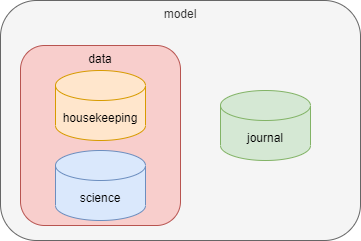
A dot notation is used to reference groups and databases. For example, moma.data.science refers to the science database in the above configuration.
Importing Data
There are several approaches for importing data into XINA, but for most projects we recommend the XINA Import utility.
XINA Import reads XINA API calls from JSON files and passes them to the XINA server. Each JSON file corresponds to a single API action, but may be paired with additional files of other types depending on the content.
For example, to upload some housekeeping data from a CSV requires two files. First, the JSON file:
{
  "action": "load",
  "database": "demo.model.data.hk.full",
  "columns": true,
  "delimit": ",",
  "line": "\n",
  "$object_id": "{local}/hk.csv"
}
The CSV file then looks like:
t,name,value
1602086313288000,SCAN_INDEX(Step),-1
1602086313288000,MO1_LD1_CURR(mA),0
1602086313288000,MO1_LD2_CURR(mA),0
1602086313288000,MO1_CASE_TEC(C),21.739
...
A couple notes on these:
- The
"line"property in the JSON file must exactly match the new line character(s) in the CSV file. You can use"\r\n"if you prefer, but either way we recommend explicitly using one or the other when you write the files, as a general "print line" may use different output depending on the platform. - The
"{local}"in the"$object_id"property is a macro used by the XINA Import application to look for the CSV file in the same location as the JSON file. We recommend using this and keeping the files in the same location. If you need to separate them you can use a full path instead, but this is more fragile if folder organization needs to be changed. - For best performance we recommend paging the CSV files so that each is 50MB or less.
- If you need to represent an empty value, you can either omit a data point or use
"NULL"(without quotes). ("NaN"and"Infinity"are not supported at the database level.)
While this CSV approach is recommended for large data sets, data can alternatively be embedded directly in JSON files. For example, a file to insert a new instant might look like:
{
  "action": "insert",
  "database": "demo.model.data.ins",
  "records": [
    {
      "u_id": "58ea870a-52c3-33c7-b858-c20795ec3301",
      "p_id": 0,
      "s_id": 0,
      "type": 20,
      "level": 0,
      "t": 1606333792000000,
      "label": "SPECTRA_Startf-0_Stopf-1k",
      "content": "some additional text here...",
      "meta": {
        "Resolution Bandwidth": 2.07014,
        "Stop Frequency": 1000,
        "Average Factor": 30,
        "Start Frequency": 0
      }
    }
  ]
}
The full API reference can be found here.
Data Types
XINA has a fixed set of data types which apply to attributes and fields. They are intended to provide consistent behavior across MySQL, Java, and JavaScript data types.
Numeric Types
Numeric data types form the backbone of most XINA data sets. Particularly in high data volume environments it is worth considering the smallest byte size type needed, as storage savings and query performance impacts can be considerable.
int(n)
Signed integer values:
| Type | Java | MySQL | JavaScript | Notes |
|---|---|---|---|---|
int(1) |
byte |
tinyint |
number |
1 byte signed integer, -27 to 27-1 |
int(2) |
short |
smallint |
number |
2 byte signed integer, -215 to 215-1 |
int(4) |
int |
int |
number |
4 byte signed integer, -231 to 231-1 |
int(8) |
long |
bigint |
number |
8 byte signed integer, -263 to 263-1 ⚠️ |
⚠️ In JavaScript number primitives are stored as an 8 byte float, so only -253 to 253-1 is available with exact precision when working in a JavaScript client (including the XINA web application).
An error is returned if a value provided is outside the range a required type, or contains a fractional value.
float(n)
Standard floating point values:
| Type | Java | MySQL | JavaScript | Notes |
|---|---|---|---|---|
float(4) |
float |
float |
number |
IEEE 754 4 byte floating point |
float(8) |
double |
double |
number |
IEEE 754 8 byte floating point |
An error will be returned if a floating point value is provided outside the representable magnitude of the required type. (Some languages denote this as Infinity/-Infinity, but this is not supported in XINA). XINA also does not recognize a NaN (not a number) floating point literal.
Boolean Type
Simple true / false type.
| Type | Java | MySQL | JavaScript |
|---|---|---|---|
boolean |
boolean |
tinyint |
boolean |
Note that MySQL treats 0 as false, non-zero as true.
Character Types
Character data types are used to store text information.
| Type | Java | MySQL | JavaScript | Notes |
|---|---|---|---|---|
utf8string(n) |
string |
char(n) |
string |
n up to 128, uses n*4 bytes, normalized |
utf8vstring(n) |
string |
varchar(n) |
string |
n up to 128, uses up to n*4 bytes, normalized |
utf8string |
string |
mediumtext |
string |
up to 224 bytes, normalized |
utf8text |
string |
mediumtext |
string |
up to 224 bytes, not normalized |
utf8filename |
string |
varchar(255) |
string |
uses up to 255 bytes, file-safe characters only |
asciistring(n) |
string |
char(n) |
string |
n up to 256, uses n bytes, normalized |
asciivstring(n) |
string |
varchar(n) |
string |
n up to 256, uses up to n bytes, normalized |
asciistring |
string |
mediumtext |
string |
up to 224 bytes, normalized |
asciitext |
string |
mediumtext |
string |
up to 224 bytes, not normalized |
asciifilename |
string |
varchar(255) |
string |
uses up to 255 bytes, file-safe characters only |
Note, all string operations are case-insensitive by default. This can be overridden with the COLLATE expression by specifying a binary collation.
Character Encoding
XINA offers two types of character encoding:
UTF-8
UTF-8 is the recommended default encoding. It has a variable length of 1 to 4 bytes per character.
ASCII
ASCII is recommended for high volume datasets where storage or indexing is critical. It is a subset of UTF-8 with a fixed length of 1 byte per character.
SQL Types
MySQL provides several types for character data storage with different considerations.
char(n)
- data stored in the table
- fixed amount of space per row (n * max_bytes_per_character)
- fastest search and index
- requires most storage
varchar(n)
- data stored in the table
- variable amount of space per row (up to n * max_bytes_per_character)
- fast search and index
text
- data stored outside the table
- slowest search and index
- only as much storage as needed
Categories
string
Text is normalized before insertion:
- leading and trailing whitespace is trimmed
- all internal whitespace is reduced to a single space character
text
Text is kept exactly as input, preserving all whitespace.
filename
Text is normalized before insertion. Content is invalid if it contains common unsafe file characters or patterns. Specifically, it is checked against the following rules:
- 255 characters or less
- Must not end with a period
- Must not match a set of Windows-specific restricted names:
-
(?!(aux|clock\\$|con|nul|prn|com[1-9]|lpt[1-9])(?:\\.|$))
-
- Must only contain upper/lower case letters, digits, space, or the characters
.-[]()$+=;#@~,&.
These rules are more restrictive than certain platforms, but are intended to provide a safe common baseline.
Temporal Types
Temporal data types store time data.
Instant
Instant types identify specific moment in time, independent of time zone. The value is stored in the database in Unix time, in one of three resolutions:
| Type | Java | MySQL | JavaScript |
|---|---|---|---|
instant(s) |
DateTime |
bigint |
date |
instant(ms) |
DateTime |
bigint |
date |
instant(us) |
DateTime |
bigint |
date |
Additionally, XINA supports standalone date and time components of instants:
| Type | Java | MySQL | JavaScript |
|---|---|---|---|
date(s) |
XDate |
bigint |
date |
date(ms) |
XDate |
bigint |
date |
date(us) |
XDate |
bigint |
date |
time(s) |
LocalTime |
int |
number |
time(ms) |
LocalTime |
int |
number |
time(us) |
LocalTime |
bigint |
number |
The date types are stored as the instant at start of date in UTC, as Unix time. The time types are stored as their respective unit limited to less than 24 hours.
XINA contains the following redundant legacy types, which will deprecated in a future release:
| Type | Java | MySQL | JavaScript | Notes |
|---|---|---|---|---|
datetime |
DateTime |
bigint |
date |
replaced by instant(ms) |
date |
XDate |
bigint |
date |
replaced by date(ms) |
time |
LocalTime |
int |
number |
replaced by time(ms) |
Instant Parsing
Instant types support parsing from either Unix time or ISO style formatted timestamps. The general goal is to allow as many formats as possible while avoiding ambiguity.
Unix Parsing
A value provided as a JSON number will be interpretted with automatic precision detection based on the following rules:
-
n > 1e16→ nanoseconds -
n > 1e14→ microseconds -
n > 1e11→ milliseconds -
n > 1e8→ seconds -
n <= 1e8→ error
This approach allows time values in the range of roughly 1973 to 5138.
A string value will be treated as Unix time if it matches the following format:
-
[+-]?(optional sign) -
\d[\d,]*(digit followed by zero or more digits or commas) -
(\.\d*)?(optional period followed by zero or more digits) -
(e[+-]?\d[\d,]*)?(optional exponent) -
([mun]?s)?(optional precision)
Examples:
-
1609459200→ 2021-01-01T00:00:00Z (auto-detected as seconds) -
1,609,459,200→ 2021-01-01T00:00:00Z (auto-detected as seconds, commas permitted and ignored) -
1609459200s→ explicit seconds -
1609459200000ms→ milliseconds -
1609459200000000us→ microseconds -
1609459200000000000ns→ nanoseconds -
0→ error (outside range supported by auto-detection) -
0s→ 1970-01-01T00:00:00Z -
−31536000s→ 1969-01-01T00:00:00Z
ISO Parsing
String values not matching the numeric format described above will be parsed as permissive ISO style formatted timestamps with an explicit offset. The ISO formats are detailed below in the local types section. The offset can be provided as:
-
±[hh]:[mm] -
±[hh][mm] -
±[hh] -
Z(UTC shorthand)
Local
Local temporal types store values as ISO 8601 formatted strings without a time zone. This has the advantage of being plain-text searchable.
| Type | Java | MySQL | JavaScript | Format |
|---|---|---|---|---|
localdate |
LocalDate |
char(10) |
string |
yyyy-MM-dd |
localtime(s) |
LocalTime |
char(8) |
string |
HH:mm:ss |
localtime(ms) |
LocalTime |
char(12) |
string |
HH:mm:ss.SSS |
localtime(us) |
LocalTime |
char(15) |
string |
HH:mm:ss.SSSSSS |
localdatetime(s) |
LocalDateTime |
char(19) |
string |
yyyy-MM-ddTHH:mm:ss |
localdatetime(ms) |
LocalDateTime |
char(23) |
string |
yyyy-MM-ddTHH:mm:ss.SSS |
localdatetime(us) |
LocalDateTime |
char(26) |
string |
yyyy-MM-ddTHH:mm:ss.SSSSSS |
localdate and localdatetime(*) are directly comparable in the database. A localdate and localtime(*) can be merged into a localdatetime(*) with CONCAT([localdate], 'T', [localtime]).
XINA contains the following redundant legacy types, which will deprecated in a future release:
| Type | Java | MySQL | JavaScript | Notes |
|---|---|---|---|---|
localtime |
LocalTime |
char(12) |
string |
replaced by localtime(ms) |
localdatetime |
LocalDateTime |
char(23) |
string |
replaced by localdatetime(ms) |
Local Parsing
Local date and time parsers use a strict resolution style with ISO chronology to ensure date validity (e.g., February 30th would be rejected). Additionally, all parsers support multiple separator characters for maximum flexibility:
-
Date separators:
-,_,. -
Time separators:
:,_,. -
Date-time separators:
T,_,. -
Fraction separators:
.,_,,
Note that local types are stored in the database in the standard ISO format regardless of the import format.
Date Parsing
Dates can be parsed from the standard ISO format:
-
Pattern:
YYYY[separator]MM[separator]DD -
Separators:
-,_,. -
Examples:
-
2011-12-03(standard ISO) -
2011_12_03(underscore) -
2011 12 03(space) -
2011.12.03(period)
-
Or an ordinal (day-of-year) ISO format:
-
Pattern:
YYYY[separator]DDD -
Separators:
-,_,. -
Examples:
-
2011-124(124th day of 2011) -
2011_124 -
2011 124 -
2011.124
-
Time Parsing
-
Pattern:
HH[sep]MM[sep]SS[frac_sep]SSSSSSSSS -
Time Separators:
:,_,. -
Fraction Separators:
.,_,, - Optional components: seconds, fractional seconds (0-9 digits)
-
Examples:
-
10:15(hour and minute only) -
10:15:30(with seconds) -
10:15:30.123456789(with nanoseconds) -
10_15_30(underscore separator) -
10.15.30,123(mixed separators)
-
Datetime Parsing
Combines local date and local time parsers.
Again, this supports standard ISO format:
-
Pattern:
{LOCAL_DATE}[date_time_separator]{LOCAL_TIME} -
Date-Time Separators:
T,_,. -
Examples:
-
2011-12-03T10:15:30(standard ISO) -
2011-12-03T10:15:30.123456789(with nanoseconds) -
2011_12_03_10_15_30(all underscores) -
2011-12-03 10:15:30(space separator) -
2011.12.03.10.15.30(all periods)
-
Or an ordinal (day-of-year) ISO format:
-
Pattern:
{ORDINAL_DATE}[date_time_separator]{LOCAL_TIME} -
Examples:
-
2011-124T10:15:30(ordinal date) -
2011_124_10_15_30 -
2011-124 10:15:30.123
-
Duration
Duration types contain a postive or negative integer duration of a specified unit.
| Type | Java | MySQL | JavaScript |
|---|---|---|---|
duration(s) |
Duration |
bigint |
number |
duration(ms) |
Duration |
bigint |
number |
duration(us) |
Duration |
bigint |
number |
JSON Types
JSON data types store JSON data directly in the database.
| Type | Java | MySQL | JavaScript |
|---|---|---|---|
jsonarray |
JsonArray |
json |
array |
jsonobject |
JsonObject |
json |
object |
Enum Types
Enum types map a series of discrete numeric integer values to text names. Though additional values may be added in the future, existing values will not change names or IDs.
notification_level
| ID | Name | Notes |
|---|---|---|
0 |
none |
default level, no associated formatting |
1 |
success |
green |
2 |
info |
cyan |
3 |
notice |
yellow |
4 |
warning |
red |
5 |
primary |
blue, elevated over none |
6 |
secondary |
grey, below none |
notification_type
| ID | Name | Notes |
|---|---|---|
0 |
post |
|
1 |
task |
|
2 |
request |
request received |
3 |
response |
response to request received |
post_level
| ID | Name | Notes |
|---|---|---|
0 |
none |
default level, no associated formatting |
1 |
success |
green |
2 |
info |
cyan |
3 |
notice |
yellow |
4 |
warning |
red |
5 |
primary |
blue, elevated over none |
6 |
secondary |
grey, below none |
System Types
ID
Wall ID
Path
Structured Data Types
UUID
HTML
XML
Collection Types
List
Set
Null Value
Although not a discrete XINA data type, null values may appear in any type depending on the context.
| Type | Java | MySQL | JavaScript | JSON |
|---|---|---|---|---|
null |
null |
NULL |
null |
null, "" (empty string) |
Broadly, the XINA interpretation of a null value is simply "no value". For this reason XINA treats empty strings in JSON as equivalent to null (because they contain no actual information). The implication of this concept in SQL is that operations on null values return null:
-
null + 1→null -
null == null→null
Record Formatting
UNDER CONSTRUCTION, details may change
A record can be formatted to a string by wrapping each field name in brackets. For example, the record:
{ "foo": "bar" }
with the format:
"Foo: {foo}"
would resolve to "Foo: bar".
Additionally, values can be passed through pipes, allowing custom formatting to be used, or modifying the value entirely. The pipe format is:
| @<pipe name> <pipe args>
Sandbox Quick Start Guide
In order to streamline onboarding for new XINA projects we have created a XINA "Sandbox" environment to test data pipelines and tools. Everything in the sandbox is fully configured as a typical XINA production environment.
Step 1: Request NAMS Access
To get started, first request access through the NAMS service. The application name is "GSFC XINA Sandbox".
Step 2: First Login
Once you receive confirmation that the account is approved, perform your first login to the XINA Sandbox by going to sandbox.xina.io. This initial login creates your user account. You will initially have access to a series of default Sandbox data. If you require access for a specific project contact our team and we will help finish setting up required permissions.
Step 3: Create an API Key
To access the XINA API for importing data you will require a XINA API key. In the XINA web application, click your user name in the top right, then "User Profile" in the drop down.

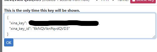
Switch to the "Access Keys" tab and click "Create New Key".

Copy the entire displayed text and save it to a local file in your preferred location. You will need to reference this file when opening the XINA Tunnel to use the XINA API. A common naming convention is <mission>_xina_key.json. The key will only be displayed once upon creation, if lost you will need to make a new key.
Step 4: Download XINA Tunnel and XINA Import
The XINA Tunnel and XINA Import utilities are the recommended starting point for importing data. Details for each are available on their respective wiki pages.
Step 5: Import Sample Data
UNDER CONSTRUCTION
Spectra Quickstart
XINA Structs includes dedicated support for spectra data files (or basically any numeric XY data plotting). Spectra data is stored in files attached to event records.
Getting Started
Once the Sandbox Quick Start Guide is complete, you can create a new model in the Sandbox project, and then a new spectra database in that model.
Create Model
{
  "action": "struct_create",
  "create": "model",
  "parent": "sandbox",
  "name": "model_name",
  "label": "Model Name",
  "desc": "example model",
  "group_teams": ["sandbox", "sandbox_dev"],
  "database_teams": ["sandbox", "sandbox_dev"]
}
Note that for this example we use "model_name" as the name of the model, so if using a different name substitute anywhere "model_name" is used in the following examples.
Create Spectra Database
Finally, create a new event file database to hold the spectra. This is an example using many of the spectra-specific features:
{
  "action": "struct_create",
  "create": "event",
  "type": "file",
  "group": "sandbox.model_name",
  "name": "spectra",
  "label": "Spectra",
  "desc": "spectra",
  "singular": "spectrum",
  "plural": "spectra",
  "teams": [ "sandbox", "sandbox_dev" ],
  "fields": [
    {
      "name": "test_stage",
      "label": "Test Stage",
      "type": "asciivstring(64)",
      "nul": true
    },
    {
      "name": "group_id",
      "label": "Group ID",
      "type": "asciivstring(128)",
      "nul": true
    },
    {
      "name": "active_mo",
      "label": "Active MO",
      "type": "asciivstring(8)",
      "nul": true
    },
    {
      "name": "active_pa",
      "label": "Active PA",
      "type": "asciivstring(8)",
      "nul": true
    },
    {
      "name": "optical_axis",
      "label": "Optical Axis",
      "type": "asciivstring(8)",
      "nul": true
    },
    {
      "name": "osa_confs",
      "label": "OSA Configurations",
      "type": "asciivstring(8)",
      "nul": true
    },
    {
      "name": "pa_current_sp",
      "label": "PA Current Setpoint",
      "type": "float(8)",
      "unit": "mA",
      "nul": true
    },
    {
      "name": "lom_temp",
      "label": "LOM Temperature",
      "type": "float(8)",
      "unit": "C",
      "nul": true
    },
    {
      "name": "peak_wavelength",
      "label": "Peak Wavelength",
      "type": "float(8)",
      "unit": "nm",
      "nul": true
    },
    {
      "name": "peak_amplitude",
      "label": "Peak Amplitude",
      "type": "float(8)",
      "unit": "dBm",
      "nul": true
    },
    {
      "name": "sidemode_lo_wavelength",
      "label": "Sidemode Lo Wavelength",
      "type": "float(8)",
      "unit": "nm",
      "nul": true
    },
    {
      "name": "sidemode_lo_amplitude",
      "label": "Sidemode Lo Amplitude",
      "type": "float(8)",
      "unit": "dBm",
      "nul": true
    },
    {
      "name": "sidemode_hi_wavelength",
      "label": "Sidemode Hi Wavelength",
      "type": "float(8)",
      "unit": "nm",
      "nul": true
    },
    {
      "name": "sidemode_hi_amplitude",
      "label": "Sidemode Hi Amplitude",
      "type": "float(8)",
      "unit": "dBm",
      "nul": true
    }
  ],
  "conf": {
    "spectrum": {
      "charts": {
        "summary": {
          "x": [
            "t_start",
            "t_end",
            "$groupRelativeTime",
            "$groupIndex",
            "lom_temp",
            "pa_current_sp",
            "$id"
          ],
          "y": [
            "peak_wavelength",
            "peak_amplitude",
            "sidemode_lo_wavelength",
            "sidemode_lo_amplitude",
            "sidemode_hi_wavelength",
            "sidemode_hi_amplitude"
          ]
        },
        "spectrum": {
          "x": [
            {
              "field": "Wavelength (nm)",
              "label": "Wavelength (nm)",
              "source": "file"
            },
            {
              "field": "Spectral Width About Peak (GHz)",
              "label": "Spectral Width About Peak (GHz)",
              "source": "file"
            }
          ],
          "y": [
            {
              "field": "Amplitude (dBm)",
              "label": "Amplitude (dBm)",
              "source": "file"
            },
            {
              "field": "Out of Band (%)",
              "label": "Out of Band (%)",
              "source": "file"
            }
          ]
        }
      },
      "filters": [
        {
          "name": "fast",
          "label": "Fast",
          "desc": "Fast",
          "color": "green",
          "checks": [
            {
              "field": "optical_axis",
              "value": "fast"
            }
          ]
        },
        {
          "name": "slow",
          "label": "Slow",
          "desc": "Slow",
          "color": "red",
          "checks": [
            {
              "field": "optical_axis",
              "value": "slow"
            }
          ]
        },
        {
          "name": "narrow",
          "label": "Narrow",
          "desc": "Narrow",
          "color": "purple",
          "checks": [
            {
              "field": "osa_confs",
              "value": "narrow"
            }
          ]
        },
        {
          "name": "wide",
          "label": "Wide",
          "desc": "Wide",
          "color": "orange",
          "checks": [
            {
              "field": "osa_confs",
              "value": "wide"
            }
          ]
        }
      ],
      "grouping": [
        "t_start",
        "group_id",
        "test_stage",
        "active_mo",
        "active_pa",
        "optical_axis",
        "osa_confs",
        "pa_current_sp"
      ]
    }
  }
}
There's a lot happening here, so we can unpack in sections.
Basic Database Parameters
{
  "action": "struct_create",
  "create": "event",
  "type": "file",
  "group": "sandbox.model_name",
  "name": "spectra",
  "label": "Spectra",
  "desc": "spectra",
  "singular": "spectrum",
  "plural": "spectra",
  "teams": [ "sandbox", "sandbox_dev" ]
}
This is the basic database configuration. The "type": "file" indicates each record will have an associated file (the spectrum data). The "teams" determines which users have read/write access to the database, and may need to be different depending on the XINA environment.
Custom Fields
{
  "fields": [
    {
      "name": "test_stage",
      "label": "Test Stage",
      "type": "asciivstring(64)"
    },
    {
      "name": "group_id",
      "label": "Group ID",
      "type": "asciivstring(128)",
      "nul": true
    },
    {
      "name": "active_mo",
      "label": "Active MO",
      "type": "asciivstring(8)",
      "nul": true
    },
    {
      "name": "active_pa",
      "label": "Active PA",
      "type": "asciivstring(8)",
      "nul": true
    },
    {
      "name": "optical_axis",
      "label": "Optical Axis",
      "type": "asciivstring(8)",
      "nul": true
    },
    {
      "name": "osa_confs",
      "label": "OSA Configurations",
      "type": "asciivstring(8)",
      "nul": true
    },
    {
      "name": "pa_current_sp",
      "label": "PA Current Setpoint",
      "type": "float(8)",
      "unit": "mA",
      "nul": true
    },
    {
      "name": "lom_temp",
      "label": "LOM Temperature",
      "type": "float(8)",
      "unit": "C",
      "nul": true
    },
    {
      "name": "peak_wavelength",
      "label": "Peak Wavelength",
      "type": "float(8)",
      "unit": "nm",
      "nul": true
    },
    {
      "name": "peak_amplitude",
      "label": "Peak Amplitude",
      "type": "float(8)",
      "unit": "dBm",
      "nul": true
    },
    {
      "name": "sidemode_lo_wavelength",
      "label": "Sidemode Lo Wavelength",
      "type": "float(8)",
      "unit": "nm",
      "nul": true
    },
    {
      "name": "sidemode_lo_amplitude",
      "label": "Sidemode Lo Amplitude",
      "type": "float(8)",
      "unit": "dBm",
      "nul": true
    },
    {
      "name": "sidemode_hi_wavelength",
      "label": "Sidemode Hi Wavelength",
      "type": "float(8)",
      "unit": "nm",
      "nul": true
    },
    {
      "name": "sidemode_hi_amplitude",
      "label": "Sidemode Hi Amplitude",
      "type": "float(8)",
      "unit": "dBm",
      "nul": true
    }
  }
}
These are the custom fields to include in the database, which will be used in addition to the default event database fields. A value for each field must be provided, unless "nul" is set to true.
Spectra Configuration
{
  "conf": {
    "spectrum": {
      "charts": {
        "summary": {
          "x": [
            "t_start",
            "t_end",
            "$groupRelativeTime",
            "$groupIndex",
            "lom_temp",
            "pa_current_sp",
            "$id"
          ],
          "y": [
            "peak_wavelength",
            "peak_amplitude",
            "sidemode_lo_wavelength",
            "sidemode_lo_amplitude",
            "sidemode_hi_wavelength",
            "sidemode_hi_amplitude"
          ]
        },
        "spectrum": {
          "x": [
            {
              "field": "Wavelength (nm)",
              "label": "Wavelength (nm)",
              "source": "file"
            },
            {
              "field": "Spectral Width About Peak (GHz)",
              "label": "Spectral Width About Peak (GHz)",
              "source": "file"
            }
          ],
          "y": [
            {
              "field": "Amplitude (dBm)",
              "label": "Amplitude (dBm)",
              "source": "file"
            },
            {
              "field": "Out of Band (%)",
              "label": "Out of Band (%)",
              "source": "file"
            }
          ]
        }
      },
      "filters": [
        {
          "name": "fast",
          "label": "Fast",
          "desc": "Fast",
          "color": "green",
          "checks": [
            {
              "field": "optical_axis",
              "value": "fast"
            }
          ]
        },
        {
          "name": "slow",
          "label": "Slow",
          "desc": "Slow",
          "color": "red",
          "checks": [
            {
              "field": "optical_axis",
              "value": "slow"
            }
          ]
        },
        {
          "name": "narrow",
          "label": "Narrow",
          "desc": "Narrow",
          "color": "purple",
          "checks": [
            {
              "field": "osa_confs",
              "value": "narrow"
            }
          ]
        },
        {
          "name": "wide",
          "label": "Wide",
          "desc": "Wide",
          "color": "orange",
          "checks": [
            {
              "field": "osa_confs",
              "value": "wide"
            }
          ]
        }
      ],
      "grouping": [
        "t_start",
        "group_id",
        "test_stage",
        "active_mo",
        "active_pa",
        "optical_axis",
        "osa_confs",
        "pa_current_sp"
      ]
    }
  }
}
Finally, the "conf" object contains the information required for XINA to interpret the event database as a spectra database. This contains three sections.
Charts
The charts section contains two subsections, "summary", and "spectra". The summary chart is displayed on the top of the Spectra Tool and plots one data point per spectrum. The configuration specifies the fields which should be listed as selectable options for the X and Y axes. This can include any of the event database default fields and/or custom fields. It also may include macros, indicated by starting with the $ character. These add additional logic and are implemented in the spectra tool itself.
The spectra chart is displayed at the bottom of the tool, and plots the full set of data for each selected spectrum. The options for each axis must be defined here to be correctly located in the associated file.
Other Features
The "filters" section defines filter options that will appear on the spectra tool, and the "grouping" option defines which fields should be available as options to create spectra groupings in the summary chart. More info on other settings is available here.
Spectrum Data Files
The spectrum files may either use a JSON format or DSV format. More formats may be added in the future.
JSON Format
A spectrum JSON file must contain a single JSON object, where each member should have an array of the same length of numeric values. An example compatible with the above spectra database could look like:
{
 "Wavelength (nm)": [ 1, 2, 3 ],
 "Spectral Width About Peak (GHz)": [ 0, 1, 0 ],
 "Amplitude (dBm)": [ 100, 200, 300 ],
 "Out of Band (%)": [ 5, 6, 7 ],
 "Comment": "ignored"
}
Note that the keys for each array must exactly match the names in the spectra "conf" object, or they will not be recognized correctly. Keys may be included which are not listed there, but they will be ignored for data purposes.
DSV Format
The spectrum DSV file format is based on the standard XINA Structs DSV file format, but doesn't require a time field. For example, a file with the same data as the above JSON example could look like:
# ignored comment
Wavelength (nm), Spectral Width About Peak (GHz), Amplitude (dBm), Out of Band (%)
1, 0, 100, 5
2, 1, 200, 6
3, 0, 300, 7
Modifications
A number of actions are available for changing the structure of a spectra database.
Drop
The drop action can delete an entire database (or group/model). This is permanent and deletes all data within the database as well, but is useful during initial experimentation as it gives a clean slate.
Drop Group
{
  "action": "drop",
  "drop": "group",
  "group": "sandbox.model_name",
  "drop_children": true
}
Note that when dropping a group, the "drop_children" flag must be true if the group contains any child groups or databases. In doing so all child groups and databases (and all data within) are deleted permanently.
Drop Database
{
  "action": "drop",
  "drop": "database",
  "database": "sandbox.model_name.spectra"
}
Reset Action
The reset action deletes all data in a database permanently. This is the fastest way to clear a database.
{
  "action": "reset",
  "database": "sandbox.model_name.spectra"
}
Altering Fields
Fields can be added or removed using the alter actions.
Add Fields
{
  "action": "alter",
  "alter": "database",
  "op": "add_fields",
  "database": "sandbox.model_name.spectra",
  "fields": [
    {
      "name": "new_field",
      "label": "New Field",
      "type": "float(8)",
      "nul": true
    }
  ]
}
Note that when adding fields to a database containing data, "nul" should typically be set to true (since existing records won't have a value for the field).
Drop Fields
{
  "action": "alter",
  "alter": "database",
  "op": "drop_fields",
  "database": "sandbox.model_name.spectra",
  "fields": [
    "unused_field"
  ]
}
Note that any data in dropped fields is deleted permanently.
Alter Configuration
The struct_alter_database_conf action can be used to update the spectrum configuration object. Care should be used when making changes here to ensure updates align with existing/added fields, and do not reference dropped fields, or errors may occur when loading the tool. Additionally, this replaces the entire "spectrum" object, so any existing configuration must be included to be preserved.
{
  "action": "struct_alter",
  "alter": "database",
  "op": "conf",
  "database": "sandbox.model_name.spectra",
  "conf": {
    "spectrum": { ... }
  }
}