Any bug reports, feature requests, or general questions can be sent to bradley.c.tse@nasa.gov or through NASA's Microsoft Teams.
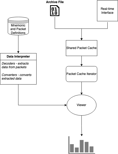
### ArchitectureThe instructions to setup the ocigse directory are maintained in the README.md of the repository: https://gs490v-gitlab.ndc.nasa.gov/497\_OCI/OCI\_XINA
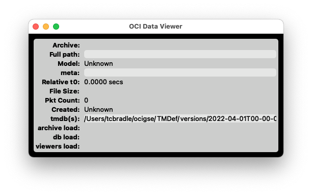
# Initial Startup When first opening the application, you will be prompted with a File Dialog and a What's New Dialog. You may close both of these. The main window (see below) displays information about the loaded archive. Depending on the operating system, the main menu may appear either at the top of the window or in the system menu bar at the top of the screen. If the menu bar is not visible, click the main window to bring it into focus.Closing this window will exit the application.
[](http://wiki.xina.io/uploads/images/gallery/2022-05/image-1651872719964.png) # Load Data ### Real-time To view data in real time: 1. Select **Setup → FEDS Client** from the menu. 2. Enter the **Instrument ID** and **FEDS Network Address** (IP address or hostname). 3. Click **Start**. 4. Verify the connection: - A confirmation message indicating a successful connection. - The **KBytes/sec** field displays a non-zero value when data is being received. - The **Pkt Count** field in the main window is incrementing --- ### Load from Archive Load archived data using one of the following File Menu options: ##### File → TID Explorer Opens a window with a tree view of the root data directory configured in `~/.699config.INI`. Clicking on a file will immediately load it. Some of the features were designed for missions that follow the TID directory naming conventions. To open the TID Explorer at startup, click the gear icon and check "Use as default". ##### File → Open Archive Opens a file selection dialog to select one or more archive files to load. The archives will be loaded in the order they are selected. ##### File → Open TID Opens a dialog to select a TID directory to load. This is intended for missions that follow the TID directory naming conventions. ##### File → Open Next TID Loads the next TID directory. This is intended for missions that follow the TID directory naming conventions. ##### File → Open Previous TID Loads the previous TID directory. This is intended for missions that follow the TID directory naming conventions. # Export Data 1. File → Export HK Data 2. Update filename 3. Select directory to export to 4. Select the column delimiter 5. The "Combine Time Columns" option will output only 1 time column. By default, there is a time column per mnemonic. 6. Select the Time Source: - Packet Time uses the time in the mission packet header. - Ground Receipt Time uses the time the ground system receives the packet. This option only works if the ground system supports it. 7. Select the Time Mode to control the format of the time column: - Relative Time is the time in seconds from the first packet's time in the loaded archive - Date/Time is the time in YYYY-MM-DD HH:MM:SS format - Timestamp is the Unix timestamp in seconds 8. Specify the Start and End Time in YYYY-MM-DD HH:MM:SS format. The default Start and End Time will encapsulate all data in the archive. 9. Click "Add Field" to select the mnemonics to export 10. Click "Export" # Clear Cached Data A configurable amount of packets are cached in memory. To clear out all cached data: Data Viewers --> Clear all data # Change the refresh rate Data Viewers --> Set Viewer Refresh Rate # Chart Tips TODO # Quick Graph You can quickly graph telemetry data over time. Data Viewers --> Quick Graph # Open a new viewer This method is used for opening up standard mission independent viewers: Data Viewers --> Viewer Finder Missions specific viewers can be opened up directly from the Data Viewers menu. The viewers listed in the last section of the Data Viewers menu are the currently open viewers. Selecting from this list will bring it to the front. # Create Tabular or Graph Viewer Data Viewers --> Make HK Viewer # OCI Viewers Instructions on how to use the various OCI viewers # DDC Raw The DDC Raw Viewer is used to display the DDC Raw captures. The DDC Raw captures are used for examining the raw samples out of the ADC. This mode is used for various tests: - Line Tune Dark - ADC Sample Point sweep - RG Mag sweep - RG Low sweep [](http://wiki2.xina.io/uploads/images/gallery/2022-04/image-1649705988672.png) # OCI Step-by-step Instructions Step-by-step instructions to use the Data Viewer for various OCI tests # ADC Sweep This page contains instructions on how to view the ADC Sweep data with the DDC Raw Viewer. The ADC sweep is performed by capturing multiple DDC raw captures while stepping the ADC sample point, which is a combination of the ADC mux delay (fine steps) and ADC Clock offset (coarse steps). One or more DDC Raw Captures may be collected at each step, depending on how the ITOS proc is configured. The collection of all steps is an "ADC Sweep". #### Setup 1. Open the DDC Raw Viewer (bring to front an existing one or open a new one) 2. Set the `CCD ID` 3. Start ADC Sweep ITOS procedure 4. The viewer will update when a complete DDC raw capture is received. A single raw capture may look something like: [](http://wiki2.xina.io/uploads/images/gallery/2022-03/image-1648764334530.png)The colored regions indicate the different parts of a "line". Each raw capture contains ~11 lines of data (dependent on various OCI settings). The "INFO" annotation indicates the start of a raw capture.
#### Sweep Finished When the ADC Sweep is finished, you may see something like below. (The actual shape may vary depending on the environment and other variables) [](http://wiki2.xina.io/uploads/images/gallery/2022-04/image-1648777610555.png) Scroll down to view the charts titled **ADC Tap** and **CDS SD Tap**. These are the main charts we will be using to analyze the ADC Sweep data. The **ADC Tap** chart displays the ADC Counts vs. ADC Sample Point, where ADC Sample Point (x-axis) is defined as: ``` ADC Sample Point = (ADC Clock Offset * 48) + Mux Delay ``` The `ADC Clock Offset` is also known as the coarse setting, `Mux Delay` as the fine setting. The **CDS SD Tap** chart displays the standard deviation of the calculated CDS for the image pixels (green region) of the 11 lines per capture.If no data is visible, you may need to rescale the chart. You can do this 1 of 3 ways: double click on the chart, right click and select "Reset zoom", or click on the number at the top right corner of the chart.
Below are a few other notes: - There is one **ADC Tap** and **CDS SD Tap** chart per tap. - You may uncheck the `Per Tap Vid/Res` setting to hide the leftmost chart - The `Sync Axes` setting will keep all of the chart axis ranges in sync. If you wish to control each chart separately, set this to `None`. - If you wish to auto scale the y-axes, check `y auto`. This will immediately rescale the y-axes, and to any new data that arrives. A common trick is to check and then uncheck to immediately rescale all of the y-axes. Note that even with `y auto` checked, the `Sync Axes` setting is still enforced which may cause unexpected behavior. At the end of the ADC Sweep, you may see something like this: [](http://wiki2.xina.io/uploads/images/gallery/2022-04/image-1648779544986.png) The **ADC Tap** charts are used to determine the ADC sample point settings we want to use. How this decision is made is outside the scope of these instructions.You may see a jump/discontinuity in the chart when going to the next coarse setting. This occurs because the actual timing delay is not continuous, but we treat and display the ADC sample point as continuous. In the below chart, you can see discontinuities at x=48 and x=96, which is where the coarse setting is incremented. This should be kept in mind when determining what sample point to use.
[](http://wiki2.xina.io/uploads/images/gallery/2022-04/image-1648782555822.png) #### Exporting - To export all of the **ADC Tap** charts as a single image, click the **Export ADC Charts** button. - To export all of the **CDS SD Tap** charts as a single image, click the **Export CDS SD Charts** button. - Each raw capture is automatically exported to disk. You can the export path in the status bar at the bottom of the window. Each raw capture is written to a single file. A corresponding hk file is exported containing relevant telemetry data for the raw capture. Unfortunately, we do not automatically group all of the raw captures for a complete ADC Sweep. You can determine this manually by using the timestamp in the filename. Zip up all relevant files for the ADC Sweep if further analysis is required. # New Page # Touch Sensitivity Test This page contains instructions on how to use the Data Viewer during the touch sensitivity tests. ##### Setup 1. Open 2 instances of the **Stats Per Pixel vs. Time** viewer. (or bring to front if already open) 2. Set the `Stats Mode` on one to `SD` and the other to `AVG`. Note: The window title displays the `Stat Mode` which can be used to differntiate the 2 instances. 3. For both configure the following settings: - `Subtrack Dark:` None - `HAM Side:` Both - `Lines mode:` All - `time win[s]:` 120 (or something reasonable) ##### Optional: - `y-auto:` check if you want the y-axis to auto scale to new data - `Sync Axes:` If enabled, the axes across the charts will be kept in sync - `Series Names:` Switch between pixel number and wavelength ##### Real-time operations: - Click the **Pause** button if you want to stop auto-scrolling the x-axis to new data - Click the **Go Live** button to resume auto-scrolling the x-axis to new data - Set the `time win[s]` to 0 to scale the x-axis to all data - If you zoom in on a chart, the x-axis auto-scrolling will be disabled if the most recent data is no longer visible on the chart. You can resume auto-scrolling by resetting the zoom or clicking the **Go Live** button. ##### No data? The charts may need to be properly scaled. Double click to zoom out, or right click and select "Reset Zoom". ##### Exporting You can export the charts as a single image by clicking on the **Snap** button. ##### Examples [](http://wiki2.xina.io/uploads/images/gallery/2022-04/image-1648787018274.png) [](http://wiki2.xina.io/uploads/images/gallery/2022-04/image-1648787048621.png) # ADC Output Phase Tuning # RG Sweeps These instructions are for the Rg Mag and Rg Low sweeps. # EMI Testing These instructions detail how to use the data viewer during EMI testing. 1. Update to get the newest EMI window config 1. Open a terminal 2. `cd ocigse` 3. `git pull` 4. Close terminal 2. On the bottom menu bar, click on `ocidataview` and select the `OCI Data Viewer` window. [](http://wiki2.xina.io/uploads/images/gallery/2022-06/image-1655400490703-27-46.png) 3. At the top of this window is a menu bar. Select `Setup` -> `Restore Windows` 4. Select `emi` and click OK. This will load the 'emi' window configuration and may take up to a minute to reload the cached data. 5. You can switch between the open viewers by clicking on the `ocidataview` in the menu bar and then selecting a viewer from the list. 6. The 4 main viewers you will be using are: - **SSM Ch Stats vs. Time - AVG** - Displays AVG counts for the whole scan per SSM channel. - **SSM Ch Stats vs. Time - SD** - Displays SD for the whole scan per SSM channel. - **Stats Per Pixel vs. Time - AVG** - Displays AVG counts for the whole scan per FPA pixel. - **Stats Per Pixel vs. Time - SD** - Displays SD for the whole scan per FPA pixel.Susceptibilities are more apparent in the SD variants; below is an example of what this may look like:
`` [](http://wiki2.xina.io/uploads/images/gallery/2022-06/image-1655774792298-25-56.png) # DDC Raw Capture Instructions to generate DDC Raw Capture images: 1. File -> Open Archives -> Select archives to open. You may select more than one. 2. Open DDC Raw viewer if not already open: Data Viewers -> DDC Raw 3. Maximize the window 4. Set settings on the right side: - CCD ID: Red or BLUE - Chart Height: 500 - Sync Axes: Both - Show Regions: checked - Line Window: 1 - Right click the "All Taps Video" chart's y-axis, set range [14500, 16500] - Right click the "All Taps CDS" chart's y-axis, set range [-50, 500] - If desired, right click on each chart and select "All series data points visible" - All other settings can be left at the defaults 5. Capture screenshot of whole window, except stop before the "All Taps Raw Samples" chart. Include the settings area on the right side. 6. Repeat as needed for RED/BLUE Below is an example screenshot: [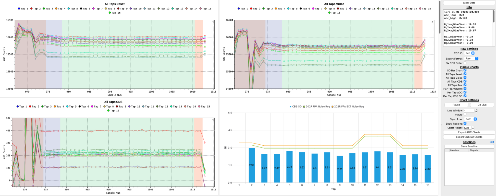](https://wiki.xina.io/uploads/images/gallery/2024-02/image-1708701901197.png) # DDC Scope Capture The DDC Scope Mode Viewer is used to view and export the collected DDC Scope Capture data. 1. File -> Open Archives -> Select archives to open. You may select more than one. 2. Open DDC Scope Mode viewer if not already open: Data Viewers -> DDC Scope Mode 3. Maximize the window 4. Any scope captures will be parsed and loaded into the "Capture List" 5. Under "Export Settings": 1. If "Auto Export Raw CSV" is checked, the raw data will be auto exported to a CSV into ~/ocidata/scope_captures/ 2. If "Auto Export Retimed CSV" is checked, the retimed data will be auto exported to a CSV into ~/ocidata/scope_captures/ 3. If "Auto Export Charts" is checked, chart images will be automatically generated to ~/ocidata/scope_captures. The y-axis for these images are scaled for dark data. For light images, you will need to manually adjust the images and then click "Export Charts". 6. The auto exported images are usually good enough for our functional tests. However, for special tests, such as performing scope captures with light, you will need to manually adjust the y-axis and export the charts by clicking "Export Charts". # Download PACE Operations Data from ODPS These instructions can be used to download PACE S-Band and OCI Ka-Band Level 0 files, which can then be loaded into the OCI Data Viewer. ##### Prerequisites: - Created an account on [https://oceandata.sci.gsfc.nasa.gov](https://oceandata.sci.gsfc.nasa.gov) - For OCI Ka-Band data, you will need to be granted access ##### Steps: 1. Navigate to [https://oceandata.sci.gsfc.nasa.gov/api/file_search/](https://oceandata.sci.gsfc.nasa.gov/api/file_search/) 2. On the left hand side above the "File Search", click "Login" and login using your credentials. Skip this step if you're already logged in. 3. Click the "Advanced" tab 4. Instrument: - For PACE S-Band Files: `PACE-spacecraft` - For OCI Ka-Band Files: `PACE-OCI` 5. Data Class: `Show All` 6. Data Type: `All` 7. Date Range: Input time range of desired data in UTC. 8. Filename Pattern (case sensitive): - For PACE S-Band Files: `HSK*HSK` - For OCI Ka-Band Files: `OCI*oci` 9. Click "Submit" 10. Click Filename to download archives Example query results for OCI files: [](https://wiki.xina.io/uploads/images/gallery/2024-02/image-1708697227300.png) # Data Viewer Usage in PACE I&T ### Overview Usage of the Data Viewer in PACE I&T has changed since we no longer receive OCI science data in real-time. OCI Science File Archives are stored on-board PACE and downlinked at a later time. OCI HK and GSE data are still received in real-time. A few updates to the Data Viewer and Science VMs have been made to accomadate for these changes. We will be running 2 instances of the Data Viewer: - One will be used to look at OCI HK and GSE data in real-time - The other will be used to open OCI Science File Archives (which also contains OCI HK data) In the bottom right of the VM, you will see 3 workspaces: [](http://wiki2.xina.io/uploads/images/gallery/2022-12/image-1671036990158.png) The **Live** workspace contains the Data Viewer that will receive OCI HK and GSE data in real-time from the FEDS. This instance of the Data Viewer works the same as in the OCI I&T environment. The **Playback** workspace contains the Data Viewer that will be used to open and view OCI Science File Archives. The **GSE** workspace contains an application that archives GSE data locally so it can be merged into the OCI Science File Archives so that OCI Science Data and GSE data can be viewed at the same time. You do not need to worry about this workspace. ### Viewing OCI Science Data To view OCI Science Data, first switch to the **Playback** workspace. Open the **Local Playback** window: - In the bottom menu bar, click on **ocidataview**. If the **Local Playback** window is already open, select it. - If not already open, select **OCI Data Viewer > Setup > Local Playback** You should see a window popup that looks like this: [](http://wiki2.xina.io/uploads/images/gallery/2022-12/image-1671037707066-08-04.png) ##### Archive Index: The **Archive Index** section on the right side displays the OCI Science File Archives that have been downlinked to the ground. You can click the **Refresh** button to refresh the list of archives. The list is also automatically refreshed the first time the **Local Playback** window is opened. This implies that the list is not automatically kept in sync with what archives have been downlinked. You may click **Load Selected Archive** to immediately open the currently selected archive. *Note: Using this method will not contain any GSE data.* ##### Playback: The **Playback** section on the left side is used for playing back time ranges of data. When you use this functionality, it will attempt to merge GSE and OCI data so that both are viewable at the same time. Selecting an archive in the **Archive Index** list will automatically update the **Start** time input. A **Duration** can be selected to choose how much data will be viewed. The max duration is 10 minutes due to resource limitations. NOTE: The **Set to most recent** is NOT aware of what data exists in the archives. It offsets from the system's current time, not the data. **Fast as possible** should generally be left checked. Once configured, click **Start** to initiate the playback. When the playback has finished, the Data Viewer will automatically load the archive. # Example Viewers ##### Raw Packet Viewer [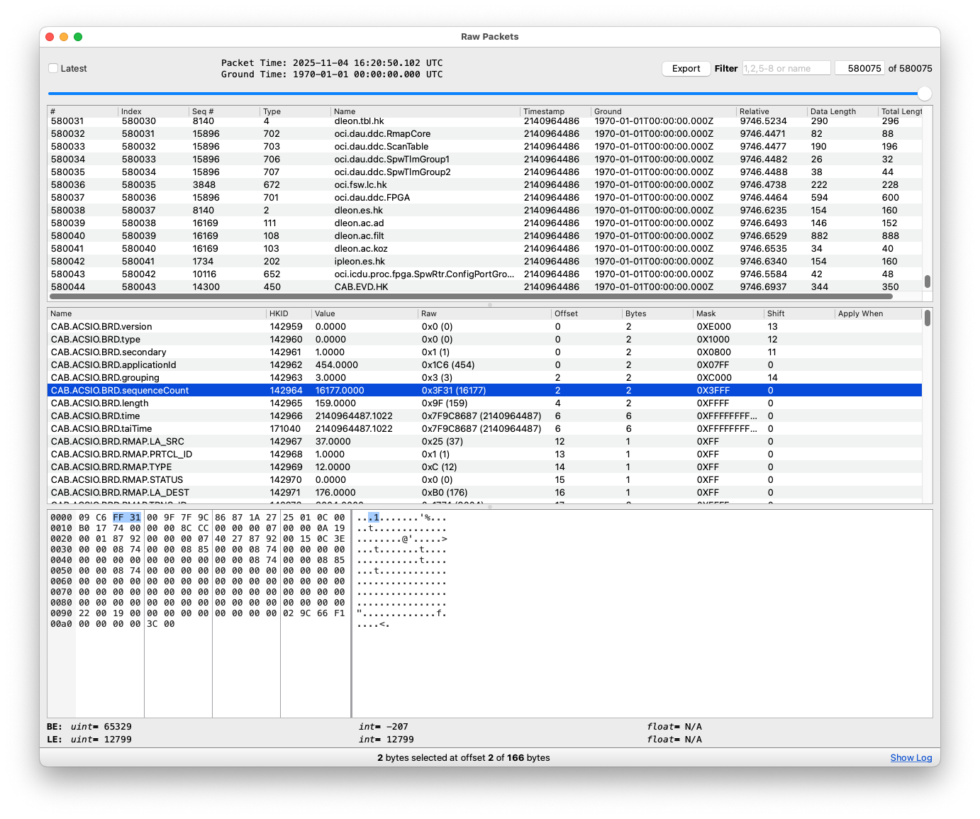](https://wiki.xina.io/uploads/images/gallery/2026-04/image-1776706636734.png) # Mnemonic Database When opening the application, the newest version of the mnemonic database is automatically loaded. You can manually load a different database with File --> Load database. # Single Page User Guide ## Table of Contents - [1. Overview](#1-overview) - [2. Install and Run](#2-install-and-run) - [2.1 Mac OS](#21-mac-os) - [2.2 Linux](#22-linux) - [2.3 Windows](#23-windows) - [2.4 Supplementary Directory](#24-supplementary-directory) - [3. Main Window](#3-main-window) - [3.1 Main Window Fields](#31-main-window-fields) - [3.2 Top Menu Bar](#32-top-menu-bar) - [4. Loading Data](#4-loading-data) - [4.1 Open a TID Directory](#41-open-a-tid-directory) - [4.2 Move Between TIDs](#42-move-between-tids) - [4.3 Open Archives](#43-open-archives) - [4.4 TID Explorer](#44-tid-explorer) - [4.5 Archive Downloader](#45-archive-downloader) - [4.6 Load a Telemetry Database](#46-load-a-telemetry-database) - [4.7 Export Housekeeping Data](#47-export-housekeeping-data) - [5. Opening Viewers](#5-opening-viewers) - [5.1 Open Viewer Files](#51-open-viewer-files) - [5.2 Viewer Finder](#52-viewer-finder) - [5.3 Make HK Viewer](#53-make-hk-viewer) - [5.4 Quick Graph](#54-quick-graph) - [5.5 Set Viewer Refresh Rate](#55-set-viewer-refresh-rate) - [5.6 Clear Viewer Data](#56-clear-viewer-data) - [6. Built-In Viewer Reference](#6-built-in-viewer-reference) - [6.1 Science and Radiance Viewers](#61-science-and-radiance-viewers) - [6.2 Counts and Statistics Viewers](#62-counts-and-statistics-viewers) - [6.3 DDC Viewers](#63-ddc-viewers) - [6.4 SSM Viewers](#64-ssm-viewers) - [6.5 GSE Viewers](#65-gse-viewers) - [6.6 Packet, Cache, Marker, and Test Viewers](#66-packet-cache-marker-and-test-viewers) - [7. Common Viewer Controls](#7-common-viewer-controls) - [8. Earth Image Workflow](#8-earth-image-workflow) - [9. Radiance vs. Time Workflow](#9-radiance-vs-time-workflow) - [10. Spectral Radiance Workflow](#10-spectral-radiance-workflow) - [11. DDC Raw Workflow](#11-ddc-raw-workflow) - [12. Saving and Restoring Windows](#12-saving-and-restoring-windows) - [13. Setup Menu](#13-setup-menu) - [14. OCI Settings](#14-oci-settings) - [15. Limits Monitor](#15-limits-monitor) - [16. Preferences](#16-preferences) - [17. Help](#17-help) - [18. Troubleshooting](#18-troubleshooting) - [18.1 No Data Appears in a Viewer](#181-no-data-appears-in-a-viewer) - [18.2 Opening a Telemetry File Fails](#182-opening-a-telemetry-file-fails) - [18.3 Archive Download Fails](#183-archive-download-fails) - [18.4 The UI Is Slow](#184-the-ui-is-slow) - [19. Documentation Maintenance Notes](#19-documentation-maintenance-notes) # 1. Overview OCI Data Viewer is an application for viewing telemetry data. It provides the following features: - View data in real-time. Supports TCP or reading from a file. - Load archives to post-process data. Supports CCSDS or 699 packets. Additional formats can be supported upon request. - Generic displays (viewers) of telemetry data: - Tabular view - Time series plots - Packet statistics - Event log - Data rate - Raw packets as hex - Custom viewers to meet a mission's needs - Generic and mission specific settings - Display science data and housekeeping telemetry data together - Save and load viewer configurations - Multiple models per mission to support per model configuration - Supports interpretation of the ITOS and ASIST mnemonic definition formats The Data Viewer can be run on Windows, Mac OS and Linux. ## 2. Install and Run ### 2.1 Mac OS Mac OS versions are distributed as an Apple Disk Image (dmg). The `dmg` contains a single `.app`which can be placed anywhere on your machine and then run. The recommended location is in your Applications directory. The `.app` contains all required dependencies. ### 2.2 Linux The Linux version is distributed as an AppImage which are similar to the Mac OS `.app`s. All dependencies are contained within the AppImage which makes it easy to distribute and run. The user or sys admin does not need to manage dependencies. The AppImage can also be run from any directory by double clicking it or running it from the terminal: ``` cdThe instructions to setup the ocigse directory are maintained in the README.md of the repository: https://gs490v-gitlab.ndc.nasa.gov/497\_OCI/OCI\_XINA
## 3. Main Window The main window displays info about the loaded data. Closing this window will close the application.  ### 3.1 Main Window Fields| Field | Description |
|---|---|
| `Archive` | Active telemetry archive file name. Blank when receiving network data. |
| `Full path` | Full path to the active telemetry file. |
| `Model` | Model associated with the data, or `Unknown` if unresolved. |
| `meta` | Metadata file path. It can identify the file, model, config, and DB patches. |
| `Relative t0` | Time origin, in seconds, used for relative telemetry times. |
| `File Size` | Current active telemetry file size, formatted as bytes, KB, MB, or GB. |
| `Pkt Count` | Number of packets currently loaded in the telemetry cache. |
| `Created` | Generated timestamp for the telemetry data, or `Unknown` if unavailable. |
| `tmdb(s)` | Loaded telemetry databases and patches used to decode, scale, and name fields. |
| `archive load` | Time required to parse and load the archive, in milliseconds. |
| `db load` | Time required to load database files and patches, in milliseconds. |
| `viewers load` | Time required to reload open viewers after data and caches are ready. |
| Viewer | Use |
|---|---|
| `Earth Image` | Build scan-line image products and export current or RGB images. |
| `Image` | View OCI image-style science data. |
| `Radiance vs. Time` | Plot radiance over time by CCD, wavelength, HAM side, and scan line. |
| `Radiance vs. Time Summed` | Plot summed radiance over time. |
| `Sci Pixel 3D` | Inspect science pixel data in a 3D visualization. |
| `Spectral Radiance` | View spectral radiance with optional FPA and SDA model overlays. |
| `Spectral Radiance Stats` | View statistical spectral radiance summaries. |
| `Spectral Waterfall` | View spectral data as a waterfall plot. |
| Viewer | Use |
|---|---|
| `Counts Per Pixel vs. Time` | Plot count data per pixel over time. |
| `Counts Per Tap (and SSM CH)` | Plot counts per tap and SSM channel data. |
| `Stats Per Pixel vs. Time` | Plot selected pixel statistics over time. |
| `Stats Per Tap vs. Time` | Plot selected tap statistics over time. |
| Viewer | Use |
|---|---|
| `DDC Func Verification` | Verify DDC functional behavior. |
| `DDC Raw` | Inspect DDC reset, video, CDS, ADC, tap, and CDS SD charts. |
| `DDC Scope Mode` | Inspect DDC scope-mode captures. |
| `DDC Sci Packet` | Inspect DDC science packets. |
| Viewer | Use |
|---|---|
| `SSM Ch Stats Table` | View SSM channel statistics in table form. |
| `SSM Ch Stats vs. Time` | Plot SSM channel statistics over time. |
| `SSM Func Verification` | Verify SSM functional behavior. |
| `SSM Line Check` | Check SSM line consistency. |
| `SSM Sci Packet` | Inspect SSM science packets. |
| `SSM Trend` | Trend SSM data over time. |
| Viewer | Use |
|---|---|
| `GSE FW Det vs. Time` | Plot GSE filter wheel detector data over time. |
| `GSE Radiance vs. Time` | Plot GSE radiance data over time. |
| `GSE Spectral Radiance` | View GSE spectral radiance data. |
| `GSE Spectral Waterfall` | View GSE spectral data as a waterfall plot. |
| Viewer | Use |
|---|---|
| `DAUC Dwell vs Time` | View DAUC dwell values over time. |
| `Markers` | View OCI markers and marker-derived context. |
| `PRBS 9` | Inspect PRBS9 verification statistics. |
| `Sci Cache` | Inspect the science cache state. |