699
General 699 pages from the archived wiki.
- 699 Software
- 699util
- 699util User Scripts
- Alerts
- Archived SAGE Versions
- BASIC Script Tools
- Bugzilla
- c699util Developer's Guide
- c699util User's Guide
- Database Patch Files
- Gnuplot
- MOMA GSE Computer Info
- Introduction to the 699 Python Library
- ISAMS
- LaTeX
- Lxml
- Melissa Trainer
- Mike Wong
- Old Main Page
- Python Performance
- Python Tool Installation
- Setup for Qt Development
- Setup Notes
- Subversion
- Supplementary Files and Telemetry File Preprocessing
- SWTS ENET User Guide
- Telemetry Database Files
- Telemetry Metadata File
- Time Synchronization Notes
- Tm2igor Quickstart
- TunnelManager
- Updating mine699
699 Software
General Information
Update Mailing List
You can sign up for the SAM Software Mailing list at https://lists.nasa.gov/mailman/listinfo/sam-software-release. Doing so will keep you notified of any software updates for XINA, SAM Data View, and Python Scripts!
Bug Reporting
Report all bugs to our Bugzilla server at https://wush.net/bugzilla/sw699/. Use the "Open a New Account" button to set up a new account. You can use this for both bug reports and feature requests.
Installation
These tools will install SAMDataview, Python 2.7, and SAM python utilities:
Mac OS X
Download and install the following files in order:
- Download the Mac OS X Python Installer from the Python.org homepage. Open the disk image and run the enclosed installer package. You will (probably) never have to update Python again, as far as SAM software is concerned. You can ignore this step when updating in the future.
- Download the source code archives of the most current distribution of 699util. Instructions for installing Python modules from source code archives can be found on that page, as well.
- Download the Mac Installer from the SAM Data View page. Open the disk image and run the enclosed installer package.
- Head to the XINA Client Install Guide page and follow the instructions to install the XINA client.
System Requirements
SAM Data View for Mac was built for Mac OS X 10.6.8, 64-bit. In our limited experience with OS X 10.7 ("Lion"), SAM Data View installs and runs with no problems, though we are not yet certain that it will work on all systems with 10.7. We do not expect a high demand for a 32-bit Mac Version of SAM Data View, but if there is, we will build a 32-bit installer. The Python tools and XINA will work on any OS (provided Python and Java, respectively, are installed).
Windows
Download and install the following files in order:
- Download the appropriate installer from the Python.org download page: Windows 32-bit or Windows 64-bit.
- Download the Windows installer from the most current distribution of 699util. Windows 7 and Vista users will need to right-click on the flie after it has downloaded and choose "Install as Administrator..."
- Head to the XINA Client Install Guide page and follow the instructions to install the XINA client.
- Download the current Windows Installer for SAM Data View (note: requires reboot after installation).
Individual Software Pages
- TunnelManager
- SAM Data View
- 699util (Python Tools)
- SAM PDS Procedure
- IGOR Software
- Developer Computer Setup
- Setup Notes (for other computers)
- Notes on Python Performance (Developers only)
- Personal User Pages:
- Melissa Trainer: IGOR scripts for atmospheric analysis
- Mike Wong: IGOR scripts for atmospheric analysis
Miscellaneous
Mac Gnuplot Installation
Short story: for legal reasons, Apple does not ship Gnu Readline library by default. The replacement library does not have all the functionality needed for gnuplot, and this often causes errors.
Download the latest Gnuplot source: http://sourceforge.net/projects/gnuplot/files/.
- Download the latest version of Gnu Readline: ftp://ftp.cwru.edu/pub/bash/readline-6.2.tar.gz.
- Untar it,
cdto the new folder, and execute./configure --prefix=/usr, thenmake everything, thensudo make install. - Then cd into the gnuplot source folder. Use
./configure,make, andsudo make install.
Mac lxml Installation
There are two big obstacles to installing lxml on a Mac. First, the Mac
standard libxml2 is often woefully out of date (at least up to 10.7;
10.8 is far better.) Therefore, in order to get a good version of
libxml2, the creators of lxml built in a way to build a static library
of libxml2 into your compilation. Unfortunately, the latest version of
libxml2 at this time of writing (2.9.0) has a bug, preventing usual
tools like "pip" from working. (If 2.9.1 is ever released, then
STATIC_DEPS=true pip install lxml will work. If you need sudo,
remember to put it between sudo and pip).
- Download The latest version of lxml from PyPi: http://pypi.python.org/pypi/lxml
- Untar it,
cdto the new folder, and executepython setup.py build --static-deps --libxml2-version=2.8.0. You may needsudopermissions, depending on your setup.
699util
This page presents a general overview of working with Python for SAM data processing tasks.
Note for SAM users: Distribution through .dmg file is no longer recommended. See PDL_Setup
Note for MOMA users: MOMA Python packages can be found at MOMA_Python_Packages.
Installation Instructions
For installation instructions, go to the Python Tool Installation page.
Bug Reports
Please do not report bugs on this wiki. Instead, use the Bugzilla server we have set up for bug tracking and reporting. Once you have set up an account, you may file a bug for the python software at the page for Command-line Utils.
List of Scripts
| Script Name | Description |
|---|---|
| checksum.py | Calculate the Fletcher's checksum of input or a list of existing files. |
| datavol.py | Estimate the data volumen of a telemetry file. |
| faradaycup.py | Correlate faraday cup scans to faraday cup currents. |
| feiget.py | Download data from FEI. |
| fei2tm.py | Convert EDRs or DPs to a telemetry file. |
| gcms.py | Print a tab-delimited table of GCMS data organized by both mass and time. |
| gcsci.py | Print GC TCD data in a tab-delimited table. |
| gcsciplot.py | Plot GC TCD data, with or without TCD offset correction. |
| getcsvreports | Script for PDL to download MSL engineering reports and sort their contents by sol. |
| hkdump.py | Print the values in a SAM type-10 housekeeping packet. |
| hot.py | Create a tab-delimited CSV file showing the cumulative number of tics the heaters have been on. |
| htrduty.py | Plot the duty cycle and temperature of a given SAM heater. |
| listfei.py | List and sort the DPs or EDRs in the current working directory. |
| massrange.py | Plot the masses and bands being scanned at a given time. |
| movefei.py | Move files downloaded from FEI into the appropriate TID folder. |
| ontime.py | Calculate how long a given component was "on" (e.g., how long a valve open, or how long an HK value was above a certain threshold) |
| phd.py | Plot the pulse-height distribution at a given marker ID. |
| powercut.py | Cut a power profile into two independent power profiles. |
| ql_ega.py | Generate the plots for a quicklook. |
| runall.py | Run a command or python code in every telemetry directory. |
| sclk2scet.py | Convert an SCLK timestamp to SCET time. |
| t0.py | Display the start time of a telemetry file in various formats. |
| timestamp.py | Print the start time of the file in a human-readable format. |
| tm2rdr.py | Create a Reduced Data Record from a telemetry file. |
| tmdb.py | A method used in backtics to get the axis name for a database entry. |
| tmdiff.py | A diff-like program for telemetry files. |
| tmdump.py | Produce a hex dump of telemetry file, packet by packet. |
| tmexcerpt.py | Create a telemetry file containing only a certain marker or packet type. |
| tmfields.py | Print a tab-delimited table of housekeeping data. |
| tmglue.py | Concatenate two telemetry files together. |
| tmkeys.py | Search for and display the telemetry database. |
| tmmarker.py | Print a list of the markers and marker IDs in the telemetry file. |
| tmmsg.py | Print the contents of the message log packets. |
| tmplot.py | Plot housekeeping data. |
| tmsanitize.py | Remove malformed data from a packet. |
| tmscan.py | Plot a DAC scan. |
| tmsequence.py | Print a report detailing whether packet sequence numbers increase normally. |
| tmstat.py | Print the statistics of a given HK value (min, median, maximum, mean). |
| tmsummary.py | Print a summary of each packet in a telemetry file. |
| triplets.py | Print a tab-delimited table of GCMS data organized by time. |
| valvestat.py | Print the valve operations (like the tmvalves viewer in SAM Data View). |
Version History
1.00.00
Source: tmutil-1.00.00.tar.gz
Release Date: 2011-11-18
- Python modules and scripts for processing telemetry data.
1.00.01
Source: tmutil-1.00.01.tar.gz
Release Date: 2011-11-22
- Updated tmenv to look for $HOME/SAM/gse/ in addition to the original $HOME/gse/ setup.
- Fixed a bug which caused the GC-specific sequence number of GC HK Packets to overwrite the packet sequence number.
1.00.02
Source: tmutil-1.00.02.tar.gz
Release Date: 2011-11-30
- Fixed bug which caused tmplot.py to crash when data was missing.
1.00.03
Source: tmutil-1.00.03.tar.gz
Release Date: 2012-12-02
- Added checksum.py script for calculating checksums of files.
- Fixed a bug which calculated the CWD for find_tmfile at the start of execution, not dynamically as the function was called.
- Made relative time default for triplets.py.
- Added regular expression-type searching for tmmsg.py, and grep-like -v (invert) option.
- Added plotref and limref scripts for LADEE EBT processing.
- Numerous bugfixes for problems observed in first round of regression testing.
1.00.04
Source: tmutil-1.00.04.tar.gz
Release Date: 2011-12-15
- Overhauled dead time correction.
- Fixed bug with showing marker IDs in tmplot.
- Fixed boot time correction for LADEE/MAVEN to avoid problems caused by race condition with time sync.
1.00.05
Source: tmutil-1.00.05.tar.gz
Release Date: 2012-01-06
- Simplified options in tmfields.py.
- Added limref
- Added plotref
- Added rf_subpacket_cal.py
- Added subpacket_timing.py
- Added on-line help for almost every script (i.e.,
-hoption)
1.00.06
Source: tmutil-1.00.06.tar.gz
Release Date: 2012-01-09
- Added background subtraction functions.
- Fixed infinite loop bug in tmread.util.step_pair.
1.00.07
Source: (missing)
Release Date: 2012-01-15
- Added newtid.py
- Added
godatacommand for the shell. - Changed sorting behavior in tmdir to use date rather than TID.
1.01.00
Source: tmutil-1.01.00.tar.gz
Release Date: 2012-03-13
- Added support for MAVEN NGMS data.
- Added lib699 package for functions not specific to telemetry.
- Added checksum.py to default distribution.
- Added massrange.py.
- Added ontime.py.
- Added t0.py.
- Added tmstat.py.
- Added tmsummary.py.
1.01.01
Source: tmutil-1.01.01.tar.gz
Release Date: 2012-03-14
- Fixed grievous errors that prevented installation.
1.02.00
Source: 699util-1.02.00.tar.gz
Revision: 66
Release Date: 2012-04-05
- Bundled TMUtil and SamUtil into 699util.
- Added support for SVN operations scripts.
- Improvements to lib699.
- Workaround to total_ordering bug in Python 2.7.1.
1.02.01
Source: 699util-1.02.01.tar.gz
Revision: 69
Release Date: 2012-05-10
- Fixed bug with setting dac mode in triplets.py.
1.02.02
Source: 699util-1.02.02.tar.gz
Revision: 88
Release Date: 2012-05-14
- Backend changes to Mission and QMS Science Packet classes.
- Incorporation of regression testing-framework (not distributed).
1.03.00
Source: 699util-1.03.00.tar.gz
Revision: 118
Release Date: 2012-05-24
- Incorporated support for time correction as a configurable file. Abandoned old concept of "offset correction."
- Added scripts for generating time configuration files from MSL-generated SCLK-SCET files.
1.03.01
Source: 699util-1.03.01.tar.gz
Revision: 150
Release Date: 2012-06-19
- Added gcsciplot.py
- Added override of Gnuplot.py's insistence on using "aqua" as the default terminal for Macs.
- Backend restructuring of feiutil.
- Added highlighting support to lib699.ttyutil and tmmsg.
- Added preliminary support for SAM Testbed.
1.03.02
Source: 699util-1.03.02.tar.gz
Revision: 167
Release Date: 2012-07-05
- Now tolerates missing SCLK/SCET file (issues a warning).
- Updates to tm2rdr.py and pds3 package.
1.04.00
Source: 699util-1.04.00.tar.gz
Revision: 326
Release Date: 2012-10-06
- Added lots of scripts, including lingering scripts that had not yet been ported to 699util and new SAM ops software
- Added lib699.collections
- Fixed svnutil performance bugs
- A little bit of Python 3 support (not fully implemented)
- tmenv moved into tmread, now uses .699config.INI file
- Added XINA SVN-post-commit hooks
1.05.00
Source: 699util-1.05.00.tar.gz (zip version: 699util-1.05.00.zip)
Windows Installer: 699util-1.05.00.macosx-10.6-intel.exe
Revision: 702
Release Date: 2013-04-17
- Too many changes to list. Incorporated every change to software since last October.
1.05.01
Source: 699util-1.05.01.tar.gz (zip version: 699util-1.05.01.zip)
Windows Installer: 699util-1.05.01.exe
Revision: 797
Release Date: 2013-05-31
- Fixed a bug with dead-time correction that causes incorrect data to be printed.
- Packet resequencing now based on packet "creation time" rather than packet timestamp.
- Fixed bug in tmfields which caused program to crash when a telemetry file did not have a defined TID.
- Many minor backend changes and bug fixes.
2.00.00
DMG (Mac) Installation Package: https://s3.amazonaws.com/699_bin/699util/699util-2.00.dmg
TAR Archive (Mac/Linux) Installation Package: https://s3.amazonaws.com/699_bin/699util/699util-2.00-installer.tar.gz
Revision: 1242
Release Date: 2013-09-05
- Now supports Python 3 instead of Python 2
- Improvements to packet parsing behavior
- Representation of time as discrete units
- Reorganization of scripts
- Streamlining of gnuplot interface
2.00.01
DMG (Mac) Installation Package: https://s3.amazonaws.com/699_bin/699util/699util-2.00.01.dmg
TAR Archive (Mac/Linux) Installation Package: https://s3.amazonaws.com/699_bin/699util/699util-2.00.01-installer.tar.gz
Revision: 1249
Release Date: 2013-09-12
- Added tm2igor.pl and igormeta.py.
- Fixed bug with ontime.py; now correctly tracks the last stretch for which a value is considered "on"
- Added samvtool alias to shell configuration script.
2.00.02
DMG (Mac) Installation Package: https://s3.amazonaws.com/699_bin/699util/699util-2.00.02.dmg
TAR Archive (Mac/Linux) Installation Package: https://s3.amazonaws.com/699_bin/699util/699util-2.00.02-installer.tar.gz
Revision: 1256
Release Date: 2013-09-13
- Added smscuplog.py.
- Full working version of nms2pds.py.
- Added nms_assemble.py.
Workaround (From Mike Wong) If
installation fails with an error of
AttributeError: \_convert while building the enum34 package, try:
Delete the tarfile enum34-1.0.tar.gz that came in the 699util*dmg disk image.
Replace it with a newer tarfile from a link such as pypi.python.org/pypi/enum34/1.1.6.
Edit the file requirements.txt, replacing "enum34==1.0" with "enum34>=1.1.6". Then try the install script again.
699util User Scripts
This page has a list of user-written scripts that aren't included in production versions of 699util. They are not guaranteed to work as the libraries get updated.
- http://s3.amazonaws.com/699_bin/userscripts/addnewfm
- http://s3.amazonaws.com/699_bin/userscripts/addtid.sh
- http://s3.amazonaws.com/699_bin/userscripts/allrev_co.sh
- http://s3.amazonaws.com/699_bin/userscripts/asist2tm.py
- http://s3.amazonaws.com/699_bin/userscripts/basicdata.py
- http://s3.amazonaws.com/699_bin/userscripts/checkout_tid.py
- http://s3.amazonaws.com/699_bin/userscripts/dacInfo.py
- http://s3.amazonaws.com/699_bin/userscripts/dacStat.py
- http://s3.amazonaws.com/699_bin/userscripts/datavol.py
- http://s3.amazonaws.com/699_bin/userscripts/deliver2sol
- http://s3.amazonaws.com/699_bin/userscripts/evrcut
- http://s3.amazonaws.com/699_bin/userscripts/fake_asist_server.py
- http://s3.amazonaws.com/699_bin/userscripts/genexpseq.pl
- http://s3.amazonaws.com/699_bin/userscripts/genvlvop.pl
- http://s3.amazonaws.com/699_bin/userscripts/hkdump.py
- http://s3.amazonaws.com/699_bin/userscripts/htr_table_dump.py
- http://s3.amazonaws.com/699_bin/userscripts/ladeecal.py
- http://s3.amazonaws.com/699_bin/userscripts/ladlib_compare.pl
- http://s3.amazonaws.com/699_bin/userscripts/ladlib_insert.pl
- http://s3.amazonaws.com/699_bin/userscripts/m50.py
- http://s3.amazonaws.com/699_bin/userscripts/m50limits.py
- http://s3.amazonaws.com/699_bin/userscripts/mavensoc2tm.py
- http://s3.amazonaws.com/699_bin/userscripts/mkdir_tid.py
- http://s3.amazonaws.com/699_bin/userscripts/mkj2000sclk.py
- http://s3.amazonaws.com/699_bin/userscripts/mkladmavsclk.py
- http://s3.amazonaws.com/699_bin/userscripts/mlfilter.sh
- http://s3.amazonaws.com/699_bin/userscripts/monchk.py
- http://s3.amazonaws.com/699_bin/userscripts/ngims_data_mining_electrodes.sh
- http://s3.amazonaws.com/699_bin/userscripts/ngims_data_mining_m50.sh
- http://s3.amazonaws.com/699_bin/userscripts/ngimsdemomine.py
- http://s3.amazonaws.com/699_bin/userscripts/penergy
- http://s3.amazonaws.com/699_bin/userscripts/pkim2limits.py
- http://s3.amazonaws.com/699_bin/userscripts/power_expand.py
- http://s3.amazonaws.com/699_bin/userscripts/pwmdump.py
- http://s3.amazonaws.com/699_bin/userscripts/ramobs.py
- http://s3.amazonaws.com/699_bin/userscripts/rf_subpacket_cal.py
- http://s3.amazonaws.com/699_bin/userscripts/samlib_compare.pl
- http://s3.amazonaws.com/699_bin/userscripts/samlib_insert.pl
- http://s3.amazonaws.com/699_bin/userscripts/scanavg.py
- http://s3.amazonaws.com/699_bin/userscripts/scet2unix.py
- http://s3.amazonaws.com/699_bin/userscripts/smshk.c
- http://s3.amazonaws.com/699_bin/userscripts/stripbas.pl
- http://s3.amazonaws.com/699_bin/userscripts/subpacket_timing.py
- http://s3.amazonaws.com/699_bin/userscripts/svnutil.py
- http://s3.amazonaws.com/699_bin/userscripts/tb_masstbl.py
- http://s3.amazonaws.com/699_bin/userscripts/tcctid.py
- http://s3.amazonaws.com/699_bin/userscripts/thermcut
- http://s3.amazonaws.com/699_bin/userscripts/timestamp.py
- http://s3.amazonaws.com/699_bin/userscripts/tmdb.py
- http://s3.amazonaws.com/699_bin/userscripts/tmenv2ini.py
- http://s3.amazonaws.com/699_bin/userscripts/tmglue.py
- http://s3.amazonaws.com/699_bin/userscripts/untunnel
- http://s3.amazonaws.com/699_bin/userscripts/xinahooktestsetup.sh
Alerts
Alerts are messages generated during mining that often serve as a notice or warning that a certain threshold or event occurred. Each alert contains a severity, a time, and a specific message.
MOMA Alerts
General Error Check
- Alert ID: 1
- Severity: Notice
- Description: Grep message log for "Error"
MAIF APV Comm
- Alert ID: 2
- Severity: Warning
- Description: Grep message log for "ldi: error"
Spacewire Comm Error
- Alert ID: 3
- Severity: Warning/Notice
- Description: Spacewire Parity (HK 522) > 0 or Spacewire Disconnect (HK 523) > 0 after 30sec
MOMA Safe Event
- Alert ID: 4
- Severity: Notice
- Description: HK 507 MAX, MOMA_STATUS_SAFE > 0 at any time during a TID
WRP Too Fast
- Alert ID: 5
- Severity: Notice
- Description: PWM Speed - HK 832 MAX > 103000
WRP Failed To Start
- Alert ID: 6
- Severity: Warning
- Description: PWM Speed - HK 832, MAX > 1000 and < 99000 RPM
WRP Pressure Spike
- Alert ID: 7
- Severity: Warning
- Description: HK 830, MOT_SUP_IMON, MAX > 1.1A
Dark Counts
- Alert ID: 8
- Severity: Warning
- Description: HK 252 SCAN_TELEM_DAC_ID = 20000 AND HK 253 SCAN_TELEM_DAC_VAL > 5
Laser Burst Energy Variation
- Alert ID: 9
- Severity: Info
- Description: Std. Dev. of burst pulse energy is > 5.0
Laser Pulses Mismatch
- Alert ID: 10
- Severity: Notice
- Description: Main Pulses != # of Pulses in Burst
Unknown SEB sequences
- Alert ID: 11
- Severity: Notice
- Description: Scan type is LDI or EI, and SEB packet sequence count == 0
Filament VMON Pegged
- Alert ID: 12
- Severity: Warning
- Description: Anytime Filament VMON HK is > 4.9
Expected Pulse Count Mismatch
- Alert ID: 13
- Severity: Warning
- Description: HKID 1050 (PLS_SUBPKT_CNT) != (pkt.length() - 4 / 16)
Gap in Scans
- Alert ID: 14
- Severity: Warning
- Description: Bin Delta between Science packets is > 100
Old Packet Format
- Alert ID: 15
- Severity: Info
- Description: Scan Packet Version Number != 2 (c_scan.science_data_pkt_version())
Missing Scan Status Packets
- Alert ID: 16
- Severity: Warning
- Description: Number of Scan Status Packets != Number of Scans in Summed Packet | Disable for Dark Counts
Dropped Packets
- Alert ID: 17
- Severity: Warning
- Description: Dropped packets are detected by gaps in the packets' sequence numbers.
Both EMs On
- Alert ID: 18
- Severity: Warning
- Description: Both Electron Multipliers are on at the same time
Sub-system Communication Errors
- Alert ID: 19
- Severity: Warning
- Description: Communication errors between any of the sub-systems (MAIF, SEB, GC, LASER) as reported by the CDH/FSW.
WRP Instantaneous High Current
- Alert ID: 20
- Severity: Warning
- Description: The instantaneous WRP Current exceeded a threshold. A Problem Report should be opened if it happened on the Flight Model.
| Mass Flow | WRP Back Pressure | Instant WRP Current |
|---|---|---|
| MP_PRESS < 0.5 | 4 Torr | 0.55 A |
| MP_PRESS < 0.5 | 6 Torr | 0.65 A |
| MP_PRESS < 0.5 | 8 Torr | 0.75 A |
| MP_PRESS > 0.5 | 4 Torr | 0.70 A |
| MP_PRESS > 0.5 | 6 Torr | 0.80 A |
| MP_PRESS > 0.5 | 8 Torr | 0.90 A |
WRP 1-Min Average High Current
- Alert ID: 21
- Severity: Warning
- Description: The 1-Min Avg WRP Current exceeded a threshold. A Problem Report should be submitted if it happened on the Flight Model.
| Mass Flow | WRP Back Pressure | 1-Min Avg WRP Current |
|---|---|---|
| MP_PRESS < 0.5 | 4 Torr | 0.45 A |
| MP_PRESS < 0.5 | 6 Torr | 0.55 A |
| MP_PRESS < 0.5 | 8 Torr | 0.65 A |
| MP_PRESS > 0.5 | 4 Torr | 0.60 A |
| MP_PRESS > 0.5 | 6 Torr | 0.70 A |
| MP_PRESS > 0.5 | 8 Torr | 0.80 A |
Archived SAGE Versions
04/18/18:
Software: SAGE1.8.3.pxp
07/18/14:
Software: SAGE1.7.pxp
11/13/13:
Software: SAGE1.6.1.pxp.zip
02/19/13:
Software: SAGE1.5.2.pxp
01/29/13:
Software: SAGE1.5.1.pxp
11/30/12:
Software: SAGE1.4.pxp
10/19/12:
Software: SAGE1.3.pxp
9/26/12:
- Fixes the peak selection cursor bug
9/24/12:
9/20/12:
Presented at the GCMS focus group meeting: SAGE_update_09_20_12.pptx
9/7/12:
8/24/12
SAM Igor tool v1.0: SAM1.0.pxp
Documentation for SAM Igor tool v1.0: SAM1.0Help.pdf
SAM IGOR previews:
BASIC Script Tools
Basic Editor
Recommended: Sublime Text
Sublime Text is a cross-platform editor, which has special features that are useful for BASIC editing. Namely, if the script and samlib.bas are open in separate tabs in the same window, Option/Command/Down Arrow will jump to the definition in samlib.bas and Ctrl - (control hyphen) will jump back to the call in the main script.
To configure syntax highlighting, install the Basic package:
Mac OS X Installation
- Press Option key and select Go/Library from Finder menu
- Navigate to Application Support/Sublime Text 3/Packages/User
- Drag "Basic" folder into this directory
- Select from language menu in lower right of Sublime window for the
relevant mission:
- User/SAM Basic
- User/MAVEN Basic
Windows Installation
- Download either the 32 or the 64 bit Windows version
- Run the executable file to install Sublime
- Relocate the contents of the "Basic" folder into: 'C:\Users\UserName\AppData\Roaming\Sublime Text 2\Packages\User'
- From the drop down menus: View>Syntax>User> SAM or MAVEN
Syntax Checker (basicyy)
Any modifications to Basic scripts should be validated using command line tool, basicyy.
Mac OS X Installation
Tested on Mac OS 10.6, 10.7, and 10.8
- Download the app package: basicyy.app package:
- Move basicyy.app into your /Applications directory
- Edit the .bash_profile file in your home directory to add a new alias:
alias basicyy="/Applications/basicyy.app/Contents/MacOS/basicyy --sam"
Omit the --sam flag if you write scripts for other missions.
In lieu of a mission flag, you may set the DEFAULT_MISSION environmental variable.
- Edit the .699config.INI file in the relevant mission section to have a script_lib_dir or script_lib_file keyword. For example:
script_lib_dir = /Users/yourname/samgse/fswTables_FLIGHT
script_lib_file = /Users/yourname/mavengse/fswTables/mavlib.940
The default is to look for the Basic library in the ScriptsCDH directory inside the gse path defined in .699config.INI.
Bugzilla
Bugzilla is the server software that the 699 team uses to help with managing our software development. It is used by both developers and users to submit bugs and enhancement/feature requests. Our server is currently being maintained by Wushnet and can be accessed here.
Creating An Account
In order to submit bug tickets or feature requests, you must first create an account. Use the "Open a New Account" button and follow the required steps.
c699util Developer's Guide
If you have not already done so, please read the c699util User's Guide to familiarize yourself with c699util and its capabilities.
This article demonstrates how to add features to c699util and describes parts of the c699util build, test, and release process. I found it challenging to create c699util due to the Qt4, 699 C++ code, SWIG, and qmake learning curves, and so I hope to ease that learning process for others. I assume that readers are familiar with Qt4 and the 699 C++ code.
SWIG
SWIG (Simplified Wrapper Interface Generator) is the program used to add a Python interface (i.e., c699util) to the 699 C++ code. As of this writing, c699util is created using SWIG 3.0.8.
Let's assume that we have code in files called example.cpp and example.hpp, and that we want to use SWIG to make this code available in Python. Our next step would be to create an interface file called example.i, and then put the declarations of the code that we want to expose to Python in that file; this is mostly just copying and pasting the declarations in example.hpp. We could then run SWIG as follows:
swig -Wall -c++ -python example.i
and SWIG would generate two files: example_wrap.cxx and example.py. example_wrap.cxx now needs to be compiled into a shared object library, and example.py will look for that shared object library when it is imported. This means that example.py is useless until example_wrap.cxx is built.
We would then build example_wrap.cxx as a dynamic library and name the resulting file _example.so (SWIG expects this naming convention -- an underscore followed by the module name. Also, there's nothing wrong with renaming a dynamic library file. These file types have no strictly enforced file extension.).
At this point, we could open up our Python interpreter and type "import example". example.py would be imported, and it would then load _example.so. example.*pp now has a Python interface.
A key takeaway from this description is that "running SWIG" successfully meant generating two files -- example.py and _example.so. Together, these two files are our new Python module.
Of course, the devil is in the details, and it's easy to make mistakes in this process. So, developers who modify c699util (or create something similar to it) are encouraged to start by making sure that they can follow this tutorial (I had to get rid of the -arch i386 flag when I went through the article), which can be thought of as the "Hello, World!" of SWIG. As with any complicated software development, a smart approach is to start with something simple that works well (such as the example in this article) and then to make small changes/enhancements to it, ensuring that the small changes work as expected.
I found the SWIG documentation and mailing list to be very helpful, particularly:
While those last two links lead to very long articles, I found it worthwhile to grit my teeth and read them in their entireties. If you find yourself maintaining c699util, you should probably do the same. However, if you're just going to make a small change to c699util, you can probably get away with just "cookbooking" off of the simpler examples in the first two links as well as existing c699util code. (If you do so, be sure to update test_c699util.py! This will be described below.)
Additionally, my personal notes on SWIG and c699util have been shared with the MOMA software team. Contact a team member if you need access.
How c699util and the 699 C++ code work together
c699util is defined in three files: c699util.cpp, c699util.hpp, and c699util.i. c699util.cpp and c699util.hpp (occasionally referred to as c699util.*pp) can be thought of as the "bridge" between the 699 C++ code and the Python scripts that want to use the features defined in the 699 C++ code. As such, c699util.*pp are responsible for hiding 699 C++ implementation details from those Python scripts. c699util.i contains the routines from c699util.*pp that we want exposed to Python; again, this is mainly done by copying declarations from c699util.hpp into c699util.i.
The general approach taken by c699util.*pp is to define a class that Python scripts expect, such as TMFile, and within that class, use 699 C++ objects to implement useful methods. For example:
class TMFile
{
public:
    // todo - I'm forgetting to use const in these methods
    TMFile(std::string filename);
    std::string filename();
    std::string absolute_directory();
    std::string directory_string();
    std::string get_mcal_filename();
    long long int file_size();
    int tid();
    int length();
    bool exists();
    TMPacket get_pkt(int index);

    double t0_in_unix_time() const;

private:
    QString filename_;
    TmMeta tmMeta_;
    MomGse::MomTelemetryFilePtr momaTlmFilePtr_;
    MomGse::MarkerCache markerCache_;
    MomGse::MomaTimestampResolver& timestampResolver_;
};
As you might expect, TMFile generates packet objects via momaTlmFilePtr_, and determines their marker and timestamp properties by using markerCache_ and timestampResolver_. TMPacket, ScienceDataCacheWrapper, and PythonStyleMomaScan follow the same design pattern.
How SWIG and qmake work together
I don't want to describe our entire build system, but there are a few c699util.pro details worth understanding:
macx {
    INCLUDEPATH += /Library/Frameworks/Python.framework/Versions/3.4/include/python3.4m
    LIBS +=        /Library/Frameworks/Python.framework/Versions/3.4/lib/libpython3.4.dylib
    INCLUDEPATH += /Library/Frameworks/QtCore.framework/Versions/4/Headers
}
linux-g++ {
    # When Python3 is installed on wherever, it should be installed with
    # "./configure --enable-shared". This is necessary so that the library files
    # generated contain position independent (-fPIC) code.
    INCLUDEPATH += /usr/local/include/python3.4m
    LIBS += /usr/local/lib/python3.4/config-3.4m/libpython3.4m.a
}
This section is the most likely to cause issues. Python can be installed in a few different ways, and in some of those ways these locations may not be valid. However, if developers install Python 3.4.3 from the Python website , then there shouldn't be any problems. Don't worry about the linux-g++ section for now. It's only for the CentOS virtual machine which is used to build c699util for mine699.
system(swig -Wall -c++ -python c699util.i)
Running qmake on the c699util.pro file invokes SWIG.
macx {
    QMAKE_LFLAGS_PLUGIN -= -dynamiclib
    QMAKE_LFLAGS_PLUGIN += -bundle
}
linux-g++ {
    QMAKE_LFLAGS_PLUGIN += -fPIC
}
When linking on OSX, replace the -dynamiclib flag with the -bundle flag, ensuring that c699util is in the Mach-O file format. I don't remember why this is necessary. When linking on the CentOS VM, produce position-independent code.
# Bundles have no strictly enforced file extension, but swig expects the
# libraries it uses to be of the form _<module name>{=html}.so , so rename the output
# file. (Don't forget the leading underscore. It's a common pitfall.)
macx {
    QMAKE_POST_LINK = "mv libc699util.dylib _c699util.so"
}
linux-g++ {
    QMAKE_POST_LINK = "mv libc699util.so _c699util.so"
}
That comment should sufficiently explain this part of c699util.pro.
How to add a feature to c699util
Getting c699util Source Code
c699util is located in svn://repos699.gsfc.nasa.gov/cppcode/qt4/trunk/c699util.
Setting up test_c699util.py
c699util/test_c699util.py is a fully automated test of c699util. I've done my best to ensure that every c699util feature is thoroughly tested inside of test_c699util.py.
So, if you find yourself modifying c699util, ensure that test_c699util.py remains a thorough test of c699util by adding good tests to it! This test suite runs on both OSX and CentOS and has saved us a lot of trouble by finding subtle bugs before our users could be affected by them. It should be run after every new feature is added to ensure that nothing else has broken (it runs in less than 60 seconds). Now, to set up your environment to run test_c699util.py, do the following:
If you have not done so, follow the instructions here to get MOMA Data View and check out MOMA data.
Now, if you have not already done so, tunnel into MOMAIOC and then open up a new tab. In this new tab, type
cd ~
svn co svn://localhost:6994/momadata/test_data ~/momadata/test_data
Then, open up any TID inside of test_data using MOMA Data View. This should add a MOMA_TEST_DATA group to your ~/.699config.INI file. Once you've done this, close MOMA Data View and open up ~/.699config.INI in a text editor. Modify this line:
[MOMA_TEST_DATA]
<other lines>
tm_database=/Users/mpallone/momagse/TMDef/MOM_TM_Database.txt
by putting "Test_" in front of MOM_TM_Database.txt. It should now look like:
[MOMA_TEST_DATA]
<other lines>
tm_database=/Users/mpallone/momagse/TMDef/Test_MOM_TM_Database.txt
This file is a copy of MOM_TM_Database.txt which has been frozen just for the sake of test_c699util.py. This way, future conversion changes to the real database won't break test_c699util.py.
Next, ensure that tmread is installed on your system.
At this point, you should have the necessary test_c699util.py dependencies. Building and running test_c699util.py is described in the next section.
Building c699util
Whenever I release a new version of c699util, I run the following commands:
make clean
qmake -spec macx-g++ c699util.pro # For CentOS, I can just run "qmake"
make release
cat top_of_c699util_dot_py.py c699util.py > temp_c699util.py && mv temp_c699util.py c699util.py
./test_c699util.py
./copy_into_699util.py # Only do this if test_c699util.py passes all tests!
(Actually, these commands are inside of the files osx_release and centos_release, and I just run one of those scripts depending on the OS I'm using.)
copy_into_699util.py is a special script which writes c699util metadata to a file called VersionInfo.txt, and then moves _c699util.so, c699util.py, and VersionInfo into their "release homes" in the 699util repository. (How c699util fits into the 699util release scheme is described later in this article; do not concern yourself with such details at this moment.) VersionInfo.txt is important because it tells software engineers who are debugging c699util (a) what version of c699util is running on a user's computer, and (b) if any uncommitted changes in the working copy made it into the user's version of c699util. Please only release c699util by using copy_into_699util.py.
Example Feature
Let's pretend that we want to add a description() method to c699util's TMPacket class. While we're at it, we'd like to make it so that calling str(pkt_object) in a Python script calls this description() method.
In c699util.hpp, we'd add the following:
/*****************************************************************************
 * TMPacket definition
 *****************************************************************************/
class TMPacket
{
public:
    TMPacket(GseLib::pbytes packetBytesPtr, int pktIndex,
             const MomGse::MarkerCache* markerCachePtr,
             const MomGse::MomaTimestampResolver& timestampResolver);

    std::string description();  // this method was just added
Next, in c699util.cpp, we would define the description() method:
/*****************************************************************************
 * TMPacket Implementation
 *****************************************************************************/

TMPacket::TMPacket(GseLib::pbytes packetBytesPtr, int pktIndex,
                   const MomGse::MarkerCache* markerCachePtr,
                   const MomGse::MomaTimestampResolver& timestampResolver)
    : packetBytesPtr_(packetBytesPtr),
      pktIndex_(pktIndex),
      markerData_(markerCachePtr->getMarker(pktIndex, &hasMarkerData_)),
      unixTimestamp_(timestampResolver.getPktUnixTime(pktIndex)),
      relativeTimestamp_(timestampResolver.getPktRelativeTime(pktIndex))
{
    // no further initialization needed
}

std::string description()
{
    return std::string("this is a description of a packet);
}
Then, in c699util.i, we would copy this declaration:
/*****************************************************************************
 * TMPacket definition
 *****************************************************************************/
class TMPacket
{
public:
    TMPacket(GseLib::pbytes packetBytesPtr, int pktIndex,
             const MomGse::MarkerCache* markerCachePtr,
             const MomGse::MomaTimestampResolver& timestampResolver);

    std::string description(); // this method was just added
    %pythoncode %{
        def __str__(self):
            return self.description()
    %}
Notice that the change we made to c699util.i is exactly the same as the
change we just made to c699util.hpp, except for the %pythoncode stuff.
(If we didn't want to add a __str__() method to TMPacket, then
c699util.hpp and c699util.i would change in exactly the same way.)
%pythoncode is a SWIG feature that allows us to define Python code that
appears in the Python file that the 'swig' command outputs (which, in
our case, is c699util.py). The __str__() method defined above will
now be a method of the TMPacket class, just as description() is a method
of the TMPacket class. Once c699util is built, calling str(pkt_object)
will invoke the __str__() method defined above, which will then call
description(). %pythoncode is an extremely useful SWIG feature because
it (a) allows us to use magical Python methods (such as generators and
iterators) that are difficult or unrealistic to implement in C++, (b)
allows us to use concise, powerful Python syntax when defining our new
classes rather than writing needlessly verbose C++ code, and (c) allows
us to import and use Python modules at runtime -- even tmread modules!
For example, consider the following uses of %pythoncode in the TMFile
class:
class TMFile

    <other TMFile methods go here>{=html}

    %pythoncode %{
        def test_name(self):
            return self.directory_string().split('-', maxsplit=5)[5]
    %}

    %pythoncode %{
        def message_log(self):
            from tmread import MessageLog
            return MessageLog(self)
    %}
Defining test_name() using %pythoncode lets take advantage of Python's
convenient string manipulation features. Defining message_log() using
%pythoncode makes it possible to use tmread's well-tested and powerful
MessageLog class, because we can import and use it at runtime.
Release Process
This process should be followed every time c699util is released. It requires a previously mentioned CentOS virtual machine, which exists solely to build and test c699util for mine699. Passwords for this VM have been distributed to the MOMA team. Copies of the VM exist on Mark Pallone's external hard drive and on the MOMA Data iMac located (as of this writing) in GSFC Building 33 F109A, ECN #2377998, inside of /Users/lab/Documents/c699util-virtual-machines.
c699util Release Process
- Update test_c699util.py so that it thoroughly tests your new feature.
- Commit the code being released.
- On your Mac, run ./osx_release. This will:
- do a clean build of c699util
- run test_c699util.py
- copy the relevant files (including working copy differences) into ~/labcode/699util/c699util, but only if the test succeeded.
- cd into ~/labcode/699util/c699util/osx, and 'svn commit' the newly built files
- On the CentOS build VM, "svn up" the momagse and qt4 directories.
- Run ./centos_release. This will:
- do a clean build of c699util
- run test_c699util.py
- copy the relevant files (including working copy differences) into ~/labcode/699util/c699util, but only if the test succeeded.
- cd into ~/labcode/699util/c699util/centos, and 'svn commit' the newly built files
- Log into mine699. On your own account (e.g., 'mpallone' instead of
the moma user):
- svn update the Python tools
- svn update ~/labcode/qt4
- cd into ~/labcode/qt4/c699util, and run test_c699util.py
- If this works, switch to the 'moma' user and update the Python tools
- Build a new Python tools package, being sure to test that the package works on our OSX VMs.
- Add a new entry to the release page.
- Commit the new DMG to
momagse/Apps/py699. - Document any new c699util features in the c699util user's guide.
- If necessary, update and release
extract_hk_data_mainon mine699 as well. (Strictly speaking this has nothing to do with c699util, but we shouldn't forget about this script when we release updates to c699util.)
It's annoying to run the test in three places, but sometimes bugs exist in one environment but not others.
c699util dependencies for both OS X and CentOS
It's useful to be aware of c699util dependencies when debugging. On OSX, _c699util.so contains the following dependencies:
(py699) gs699-mpallone:c699util mpallone$ otool -L _c699util.so
_c699util.so:
   /Library/Frameworks/Python.framework/Versions/3.4/Python (compatibility version 3.4.0, current version 3.4.0)
   QtGui.framework/Versions/4/QtGui (compatibility version 4.8.0, current version 4.8.4)
   QtCore.framework/Versions/4/QtCore (compatibility version 4.8.0, current version 4.8.4)
   QtNetwork.framework/Versions/4/QtNetwork (compatibility version 4.8.0, current version 4.8.4)
   /usr/lib/libstdc++.6.dylib (compatibility version 7.0.0, current version 104.1.0)
   /usr/lib/libSystem.B.dylib (compatibility version 1.0.0, current version 1226.10.1)
   /usr/lib/libgcc_s.1.dylib (compatibility version 1.0.0, current version 915.0.0)
The expected location of these dependencies can be tweaked by using the install_name_tool program. Python 3.4 should be in the specified location if it is installed through the DMG file available on the Python website. The use of Homebrew in this particular case is discouraged. The Qt dependencies should be discoverable once Qt4 is installed. The remaining dependencies were already available on my Mac; I suspect that they're standard on all modern Macs.
Unlike the OSX distribution of c699util, the CentOS distribution has the Python and Qt dependencies statically compiled into the _c699util.so file. The .so file's remaining dependencies are all standard (i.e., they're available by default on CentOS machines such as mine699.gsfc.nasa.gov).
c699util, the 699 developer setup, and the 699util package release scheme
Releasing c699util means committing new versions of
- c699util.py
- _c699util.so
- VersionInfo.txt
into the repos699 SVN server, in the locations
labcode/699util/c699util/osx and labcode/699util/c699util/centos.
The rest of this section describes how c699util fits into the the
699util developer's setup and the 699util package release system.
Review of the 699util Environment
Even for those who are familiar with the 699util installation article, how all the different parts of 699util fit together can still be hard to understand. So, reviewing this should make the rest of this section much easier to understand.
The 699util environment has four major parts:
- 699 Data
- 699 tool configuration/settings
- 699 Code
- Local environment configuration
1. 699 Data. Setting up 699 data simply means checking out folders
such as momadata/etu, momadata/fm, etc. from
momaioc.gsfc.nasa.gov's SVN
repository.
Typically, momadata is checked out into the home directory, but this is
not required.
2. 699 tool configuration/settings. Items in this category mainly tell 699 software where data is, and how to interpret that data. This category includes:
- checking out momagse
- using MOMA Data View to initialize the ~/.699config.INI file.
Simply open up a TID for each model that you have checked out in
your
momadataworking copy. - (If you're doing a developer install, you will also have to checkout config699.)
3. 699 code. Developers can check out 699util from SVN. Users can find MOMA script DMGs here.
4. Local environment configuration. This tends to be the most opaque. It consists of the following:
- Installing Python 3.4.3 from the Python website, and updating your .bashrc, .bash_profile, or .profile file so that the newly installed version of Python can be found via the PATH environment variable.
-
setting up a virtual environment using the program
virtualenv.
A virtual environment can be thought of as a folder containing
libraries and executable programs, as well as the environment
variables that reference those libraries and executables. In the
699util world, virtualenv is used to create either
~/py699or~/py699-moma. Python 3.4.3 is copied into this directory and, in the case of the package install, 699util scripts are also copied. Typically, the last line of a user's~/.bashrcfile "activates" the virtual environment, which essentially just puts the virtual environment's binary folder (e.g.,~/py699/bin) at the front of the PATH variable. Then, when a scripts starts with#!/usr/bin/env python3, the first instance of the python3 executable found by the/usr/bin/envprogram will be the one inside of the~/py699directory. - The location of the 699util scripts, such as tmplot.py. In the
package install meant for users (i.e., non-developers), these
scripts are simply copied into the virtual environment folder
~/py699/bin. For developers who already have these scripts checked out into a working copy, the location of those scripts is added to the PATH variable as follows:- the developer opens up a terminal
- the terminal sources the developer's
~/.bashrcfile - the
~/.bashrcfile sources the~/config699/bash_config.shfile, which adds the script directories to the PATH variable.
- The location of 699util libraries. This is very similar to how
scripts are handled. For non-developers, the 699util Python library
is in the virtual environment's library folder. For developers, the
~/config699/bash_config.shdirectory adds the libraries to the PYTHONPATH environment variable, which Python uses when looking for modules that need to be imported.
Developer Setup
As mentioned above, the developer install sources
~/config699/bash_config.sh, which sets PATH and PYTHONPATH environment
variables. bash_config.sh determines the version of c699util that's
correct for the user's operating system, and adds that directory to the
PYTHONPATH variable. More explicitly, if c699util exists in this
location:
~/labcode/699util/c699util/osx/c699util.py
~/labcode/699util/c699util/osx/_c699util.so
then the directory ${HOME}/labcode/699util/c699util/osx will be added
to the user's PYTHONPATH, so that the import c699util code inside of
a Python script can know to look in this directory.
As mentioned in a previous section, _c699util.so has some Qt4
dependencies. When `import c699util` is executed, some code at the top
of c699util.py will determine if _c699util.so's dependencies are
unresolved, and if so, change the dependencies to point to the correct
location on the user's computer.
699util Package Release
Non-developers (i.e., users) install 699util by mounting a 699util .dmg
file and running the install699util.sh script. The package release
scheme does not use the aforementioned ~/config699/bash_config.sh
script. The .dmg file contains the following in its root directory:
- _c699util.so
- 699util.py
- Qt4 dependencies
install699util.sh simply copies these files into the virtual
environment folder ~/py699/lib, and then tweaks the user's .bashrc
file so that ~/py699/lib is always in the users' PYTHONPATH whenever
a new terminal is opened.
c699util User's Guide
Similar to Introduction to the 699 Python Library, this article is a high-level description of c699util, intended for those who are only using it to write Python scripts. I do not describe low level c699util details here. For that, see the c699util developer's guide.
c699util is a Python module which provides housekeeping and science data extraction routines for MOMA telemetry files. Its interface is very similar to 699util's tmread module:
   #!/usr/bin/env python3

   #==============================================================================
   # Packet data extraction through 699util's tmread module:
   #==============================================================================
   import tmread

   tmfile = tmread.get_tmfile('/Users/mpallone/momadata/fm/2016-01-15-14.06.47-30410-MSFUNC/tm.mom.m3.s3')

   wrp_current_datapoints = []
   wrp_current_hkid = 800
   pkt_17_count = 0

   for pkt in tmfile(17):
       pkt_17_count += 1
       wrp_current_datapoints.extend(pkt[wrp_current_hkid])

   # Print out the data:
   print("pkt_17_count:", pkt_17_count)
   print()
   print("WRP current sample timestamp, WRP current sample science value:")
   for timestamp, value in wrp_current_datapoints:
       print(timestamp, 't', value)


   #==============================================================================
   # Packet data extraction through c699util:
   #==============================================================================
   import c699util

   c_tmfile = c699util.construct_tmfile('/Users/mpallone/momadata/fm/2016-01-15-14.06.47-30410-MSFUNC/tm.mom.m3.s3')

   wrp_current_datapoints = []
   wrp_current_hkid = 800
   pkt_17_count = 0

   for pkt in c_tmfile(17):
       pkt_17_count += 1
       wrp_current_datapoints.extend(pkt[wrp_current_hkid])

   # Print out the data:
   print("pkt_17_count:", pkt_17_count)
   print()
   print("WRP current sample timestamp, WRP current sample science value:")

   #for timestamp, value in wrp_current_datapoints:
   #    print(timestamp, 't', value)

   # Note the change here!
   for datapoint in wrp_current_datapoints:
       print(datapoint.relative_timestamp, 't', datapoint.value)
As this example illustrates, some minor interface differences exist between c699util and tmread, which are documented at the end of this article.
You are highly encouraged to follow the following convention: if you use c699util in a Python script, please prefix it with "c_". For example, when I ported ioncount.py over to c699util, I made a copy of ioncount.py, called it c_ioncount.py, and then replaced tmread code with similar c699util code. This way, both scripts are available to run (a nice option to have if we encounter bugs), and we always know which underlying library we're using.
If we already have tmread, why bother with c699util?
Well, for one, c699util is about an order of magnitude faster than tmread (and sometimes more -- c_ioncount.py was 39x faster than ioncount.py when extracting selected ion counts).
More importantly, much of tmread is deprecated for MOMA. Any feature that tmread shares with c699util is no longer maintained. Instead of maintaining telemetry extraction libraries in C++, and then duplicating the exact same functionality in Python, we've decided to simply add a Python interface to the C++ code. This dramatically simplifies feature implementation, eliminates consistency issues between various tools, and speeds up software development and program run time, but it also means that tmread won't output data as accurately as c699util, and also won't have as many features.
c699util Flaw -- only one TMFile at a time
Because the C++ code around which c699util wraps frequently uses singletons, c699util can only operate on one TMFile at a time. Calling c699util.construct_tmfile() will invalidate any previously existing c699util.TMFile objects.
We rarely ever (if at all) need this capability, but when the C++ and c699util code is ported over to future missions, this design should be reconsidered.
Obtaining c699util
If you do not have the 699 Python tools installed on your computer, then the developer instructions in Python_Tool_Installation should work, although it's probably best to just ask a MOMA software developer to do it for you. Be sure to install Python 3.4.3 from the Python website.
If you already have 699 Python tools installed, you will probably also have to ask a MOMA software developer to setup c699util. Most likely, Python 3.4.3 will need to be installed directly from the website (sorry, Homebrew aficionados), and your virtual environment will need to be rebuilt so that it uses Python 3.4.3. However, if you happen to already be using Python 3.4.3, then SSH tunneling into repos699 and then updating ~/config699 and ~/labcode/699util should be all that you need to do to start using c699util.
TMFile
c699util provides a TMFile class which is very similar to tmread's TMFile class. c699util.TMFile objects can be obtained as follows:
   import c699util
   c_tmfile = c699util.get_tmfile('/Users/mpallone/momadata/fm/2016-01-15-14.06.47-30410-MSFUNC/tm.mom.m3.s3')
c699util.get_tmfile() is a thin wrapper around tmread.get_tmfile(), so it does all of the telemetry-file-finding-magic that tmread.get_tmfile() does:
   import c699util
   c_tmfile = c699util.get_tmfile() # grab the tm.mom file in the cwd
   c_tmfile = c699util.get_tmfile(12345) # Grab TID 12345
   c_tmfile = c699util.get_tmfile("/Users/mpallone/momadata/fm/2016-01-15-14.06.47-30410-MSFUNC") # Grab the tm.mom file in the specified directory
It would be preferable to not use the deprecated tmread module, but it seems unlikely to me that I'll ever get around to implementing get_tmfile()'s magic inside of c699util, at least on MOMA. Also, this tactic allows us to keep using the extremely useful TMArgumentParser class.
If tmread is not available, c699util.construct_tmfile() can be used:
   import c699util
   c_tmfile = c699util.construct_tmfile('/Users/mpallone/momadata/fm/2016-01-15-14.06.47-30410-MSFUNC/tm.mom.m3.s3')
Also, note the convention of using c_tmfile. I prefer to use 'tmfile' for tmread.TMFile objects, and 'c_tmfile' for c699util.TMFile objects, so that I can tell at a glance what kind of object I'm using. I strongly recommend that other script writers do the same.
Other useful methods:
   #!/usr/bin/env python3

   import tmread, c699util
   tmfile = tmread.get_tmfile(30410) # Give it a TID and let it find the file for us
   c_tmfile = c699util.construct_tmfile(tmfile.filename)

   # (alternatively, we could just do c_tmfile = c699util.get_tmfile(30410)

   print("Absolute filename:", c_tmfile.filename())
   print("Absolute filename:", str(c_tmfile))
   # Absolute filename: /Users/mpallone/momadata/fm/2016-01-15-14.06.47-30410-MSFUNC/tm.mom.m3.s3

   print("Absolute directory:", c_tmfile.absolute_directory())
   # Absolute directory: /Users/mpallone/momadata/fm/2016-01-15-14.06.47-30410-MSFUNC

   # Parsed from the first GSE packet in the tm.mom file:
   print("TID Directory name:", c_tmfile.directory_string())
   # TID Directory name: 2016-01-15-14.06.47-30410-MSFUNC

   print("Mass calibration file used:", c_tmfile.get_mcal_filename())
   # Mass calibration file used: 2016-01-17-23.48.39-30410.mcal

   print("File size in bytes:", c_tmfile.file_size())
   # File size in bytes: 48384623

   print("TID:", c_tmfile.tid())
   # TID: 30410

   print("t0 in Unix time:", c_tmfile.t0_in_unix_time())
   # t0 in Unix time: 1452884878.3959727

   print("Number of packets:", c_tmfile.length())
   print("Number of packets:", len(c_tmfile))
   # Number of packets: 70232

   print("TMFile actually exists on the filesystem:", c_tmfile.exists())
   print("TMFile actually exists on the filesystem:", bool(c_tmfile))
   # TMFile actually exists on the filesystem: True

   pkt_at_index_10 = c_tmfile.get_pkt(10)
   pkt_at_index_10 = c_tmfile[10]

   # We can iterate through c_tmfile and get packet objects:
   pkt_count = 0
   for pkt in c_tmfile:
       pkt_count += 1

   # The old tm_filter routines also work for c699util:
   pkt_17_count = 0
   for pkt in c_tmfile(17):
       pkt_17_count += 1

   pkt_count = 0
   for pkt in c_tmfile(type_filter=17,      # Only yield packets of type 17
                       marker_filter=2500,  # Only yield packets at marker 2500
                       start_time=1000,     # Relative time = 1000 seconds
                       stop_time=2000):     # Relative time = 2000 seconds
       pkt_count += 1

   # If the directory name is
   #     '2016-01-15-14.06.47-30410-MSFUNC'
   # then the test name is
   #     'MSFUNC'
   print("Test name:", c_tmfile.test_name())

   # tmread.MessageLog is not deprecated, and is fully compatible with c699util:
   msg_log = c_tmfile.message_log()

   meta_markers = c_tmfile.get_meta_markers()
   for meta_marker in meta_markers:
       print(meta_marker.startRelativeTimeInSecs)
       print(meta_marker.endRelativeTimeInSecs)
       print(meta_marker.metaMarkerId)
       print(meta_marker.index)
       print(meta_marker.msg)

   print("model:", c_tmfile.model())
   # model: fm

   print("FSW timestamp at of t0 packet:", c_tmfile.t0_in_sclk())
   # FSW timestamp at of t0 packet: 19351744
tmread.extract_tmfields() is compatible with c699util.TMFile objects:
   #!/usr/bin/env python3

   import tmread, c699util
   tmfile = tmread.get_tmfile(30410) # Give it a TID and let it find the file for us
   c_tmfile = c699util.construct_tmfile(tmfile.filename)

   AUX_AMP_DAC_SET_HKID = 61
   RF_AMP_MON_HKID      = 62

   fields = tmread.extract_tmfields(c_tmfile, [AUX_AMP_DAC_SET_HKID, RF_AMP_MON_HKID])

   # Note that we still get c699util.TMDatapoint objects here, which are different
   # from 699util's tmread datapoints!
   sum_ = 0
   count = 0
   for datapoint in fields[RF_AMP_MON_HKID]:
       relative_timestamp = datapoint.relative_timestamp
       unix_timestamp = datapoint.unix_timestamp
       raw_timestamp = datapoint.fsw_timestamp
       sum_ += datapoint.value
       count += 1

   if count != 0:
       print("RF Amp mon avg:", sum_ / count)

## TMPacket

Just like TMFile, c699util provides TMPacket objects which are very
similar to tmread.TMPacket objects:

   #!/usr/bin/env python3

   import tmread, c699util
   tmfile = tmread.get_tmfile(30410) # Give it a TID and let it find the file for us
   c_tmfile = c699util.construct_tmfile(tmfile.filename)

   gse_pkt = c_tmfile[0]       # Pkt type 8, GSE generated
   pkt_22 = c_tmfile[65]       # Pkt type 22
   msg_log_pkt = c_tmfile[85]  # Pkt type 8

   print("Unmasked type of gse_pkt:", gse_pkt.full_type())
   # Unmasked type of gse_pkt: 136

   print("Unmasked type of pkt_22:", pkt_22.full_type())
   # Unmasked type of pkt_22: 22

   # This is analagous to tmread.TMPacket.type
   print("gse_pkt with gse-generated bit masked out:", gse_pkt.get_type())
   # gse_pkt with gse-generated bit masked out: 8

   print("pkt_22 length, including header and checksum:", pkt_22.total_length())
   # pkt_22 length, including header and checksum: 224
   print("pkt_22 length, just the data:", pkt_22.length())
   # pkt_22 length, just the data: 212

   print("pkt_22 checksum:", pkt_22.checksum())
   print("pkt_22 checksum:", hash(pkt_22))
   # pkt_22 checksum: 1379474455

   print("Is pkt_22 gse created?", pkt_22.gse_created())
   # Is pkt_22 gse created? False
   print("Is gse_pkt gse created?", gse_pkt.gse_created())
   # Is gse_pkt gse created? True

   print("pkt_22 sequence number:", pkt_22.sequence())
   # pkt_22 sequence number: 146

   # Yes, I'm aware that 'sclk' is a misnomer
   print("pkt_22 FSW timestamp:", pkt_22.sclk())
   # pkt_22 FSW timestamp: 19540225
   print("pkt_22 FSW timestamp, in seconds:", pkt_22.sclk_in_seconds())
   # pkt_22 FSW timestamp, in seconds: 1954.0225

   print("pkt_22 index:", pkt_22.index())
   # pkt_22 index: 65

   print("pkt_22 marker ID:", pkt_22.marker_id())
   # pkt_22 marker ID: 0

   # Packets before the first marker packet have a marker index of 0
   print("pkt_22 marker index:", pkt_22.xina_marker_index())
   # pkt_22 marker index: 0

   print("pkt_22 unix timestamp, in seconds:", pkt_22.unix_timestamp())
   # pkt_22 unix timestamp, in seconds: 1452884897.2440727

   print("pkt_22 relative timestamp, in seconds:", pkt_22.relative_timestamp())
   # pkt_22 relative timestamp, in seconds: 18.848099946975708

   print("pkt_22 marker text:", pkt_22.marker_text())
   # pkt_22 marker text: <no marker text, but you get the idea>

   ###########################################################
   #
   # (this doesn't actually work for TID 30410, but I think you get the picture)
   #
   # HKID 100 = phase cycle readback HKID
   phase_cycle_readback_raw_data = pkt_22.all_raw_data(100)
   phase_cycle_readback_eng_data = pkt_22.all_eng_data(100)

   phase_cycle_readback_sci_data = pkt_22.all_data(100)
   phase_cycle_readback_sci_data = pkt[100]

   datapoint = phase_cycle_readback_sci_data[0]
   print("Datapoint unix timestamp, in seconds:", datapoint.unix_timestamp)
   print("Datapoint relative timestamp, in seconds:", datapoint.relative_timestamp)
   print("Datapoint value:", datapoint.value)

   first_phase_cycle_readback_science_sample = pkt_22.get_first_value(100)
   #
   #
   ###########################################################

   print("Does gse_pkt have an earlier timestamp than pkt_22?", gse_pkt < pkt_22)
   # Does gse_pkt have an earlier timestamp than pkt_22? True

   print("Raw message log:", msg_log_pkt.raw_message())
   print("Sanitized message log:", msg_log_pkt.message())
   # (output omitted for brevity)

   print("raw bytes:", pkt_22.raw_packet())
   # b'x16x92x00xd4x01*)x01xfaxf3 x02x00...(etc).

   meta_markers = pkt_22.get_meta_markers()
   for meta_marker in meta_markers:
       print(meta_marker.startRelativeTimeInSecs)
       print(meta_marker.endRelativeTimeInSecs)
       print(meta_marker.metaMarkerId)
       print(meta_marker.index)
       print(meta_marker.msg)
Extracting Science Data
c699util has a get_scans() function, just like tmread.momascience:
   #!/usr/bin/env python3

   import c699util
   c_tmfile = c699util.get_tmfile(30410)

   scan_count = 0
   for scan in c699util.get_scans(c_tmfile):
       scan_count += 1

   print("Number of scans:", scan_count)
The usual packet type, marker filtering, start time, etc. filtering options are available.
Unlike tmread, c699util provides a wrapper around MOMA Data View's ScienceDataCache class:
   #!/usr/bin/env python3

   import c699util

   # Not needed
   # c_tmfile = c699util.construct_tmfile(tmfile.filename)

   # Notice that this factory function takes the absolute filename, just like
   # construct_tmfile
   # science_cache = c699util.construct_science_data_cache('/Users/mpallone/momadata/fm/2016-01-15-14.06.47-30410-MSFUNC/tm.mom.m3.s3')

   science_cache = c699util.get_science_data_cache(30410)
c699util.get_science_data_cache() is analagous to c699util.get_tmfile(), so it can be passed no arguments if the programmer wants to search the cwd, or just the TID to search for, or the absolute path of the tm.mom file, etc.
The science cache can be iterated through to get scan objects (just c699util.get_scans()), or it can be indexed, as demonstrated below.
   #!/usr/bin/env python3

   import c699util

   science_cache = c699util.get_science_data_cache(30410)

   last_scan = science_cache[-1]

   print("Last scan data:")

   print("Unix timestamp, in seconds:", last_scan.unix_timestamp())
   # Unix timestamp, in seconds: 1452890221.7956727

   print("Relative timestamp, in seconds:", last_scan.relative_timestamp())
   # Relative timestamp, in seconds: 5343.399699926376

   print("marker ID:", last_scan.marker_id())
   # marker ID: 2050

   print("marker Index:", last_scan.xina_marker_index())
   # marker Index: 136

   print("marker text:", last_scan.marker_text())
   # marker text: SCN 602 START Emission Current Source B

   list_of_ion_counts = last_scan.counts()
   print("total ion count:", sum(list_of_ion_counts))
   print("total ion count:", last_scan.total_ion_count())
   # total ion count: 40463

   print("Highest count in the last_scan:", last_scan.highest_count())
   # Highest count in the last_scan: 708

   print("Bin number containing the highest count:", last_scan.highest_count_bin_num())
   # Bin number containing the highest count: 1710

   print("Lowest count:", last_scan.lowest_count())
   # Lowest count: 0

   # There should be one entry for every 100 bins
   rf_status_entry_list = last_scan.rf_status_entries()
   rf_entry = rf_status_entry_list[0]

   print("First RF Entry start bin:", rf_entry.start_bin)
   # First RF Entry start bin: 0

   print("First RF Entry RF Amp V:", rf_entry.rf_amp_v)
   # First RF Entry RF Amp V: 66.67613871395588

   print("First RF Entry RF Amp DAC V:", rf_entry.rf_amp_dac_v)
   # First RF Entry RF Amp DAC V: 70.00512770935893

   print("First RF Entry Aux Amp DAC V:", rf_entry.aux_amp_dac_v)
   # First RF Entry Aux Amp DAC V: 1.0998702980577946

   print("RF Amp Start:", last_scan.rf_amp_start())
   # RF Amp Start: 66.67613871395588

   print("RF Amp End:", last_scan.rf_amp_end())
   # RF Amp End: 993.6579284607433

   print("RF Amp DAC Start:", last_scan.rf_amp_dac_start())
   # RF Amp DAC Start: 70.00512770935893

   print("RF Amp DAC End:", last_scan.rf_amp_dac_end())
   # RF Amp DAC End: 996.3826513544906

   print("Aux Amp DAC Start:", last_scan.aux_amp_dac_start())
   # Aux Amp DAC Start: 1.0998702980577946

   print("Total scan time, in seconds:", last_scan.total_scan_time())
   # Total scan time, in seconds: 0.05000000074505805

   print("Peak counts per second:", last_scan.peak_counts_per_sec())
   # Peak counts per second: 70799998.9449978

   print("Pkt source type (26 or 27):", last_scan.src_pkt_type())
   # Pkt source type (26 or 27): 27

   print("Number of scans that went into this scan (typically 10 for sum packets):")
   print(last_scan.num_scans())
   # Number of scans that went into this scan (typically 10 for sum packets):
   # 10

   print("Does this scan have a scan status packet?", last_scan.has_scan_status())
   # Does this scan have a scan status packet? True

   print("Number of scan status packets:", last_scan.num_scan_status_pkts())
   # Number of scan status packets: 10

   print("Does this scan have a preceding SEB HK packet?", last_scan.has_seb_hk_pkt())
   # Does this scan have a preceding SEB HK packet? True

   print("Is this scan a dark count scan?", last_scan.is_dark_count_scan())
   # Is this scan a dark count scan? False

   print("Sum of the ion counts for bins 500-600:")
   print(last_scan.selected_ion_count_sum_by_bin(500,600))
   # Sum of the ion counts for bins 500-600:
   # 3981

   print("Sum of the ion counts between masses 138-140:")
   print(last_scan.selected_ion_count_sum_by_mass(138,140))
   # Sum of the ion counts between masses 138-140:
   # 78

   print("Maximum ion count between bins 500-600:")
   print(last_scan.selected_ion_count_max_by_bin(500,600))
   # Maximum ion count between bins 500-600:
   # 537

   print("Maximum ion count between masses 138-140:")
   print(last_scan.selected_ion_count_max_by_mass(138,140))
   # Maximum ion count between masses 138-140:
   # 21

   print("seb_bin_time_readback:", last_scan.seb_bin_time_readback())
   # seb_bin_time_readback: 10.000000149011612

   print("seb_bin_time_readback_in_seconds:", last_scan.seb_bin_time_readback_in_seconds())
   # seb_bin_time_readback_in_seconds: 1.0000000149011612e-05

   print("seb_special_scan_id:", last_scan.seb_special_scan_id())
   # seb_special_scan_id: 602

   print("seb_raw_scan_value:", last_scan.seb_raw_scan_value())
   # seb_raw_scan_value: 127

   print("seb_scan_value:", last_scan.seb_scan_value())
   # seb_scan_value: 49.80392238497734

   print("seb_rf_freq_hz:", last_scan.seb_rf_freq_hz())
   # seb_rf_freq_hz: 988400.0

   print("seb_last_rf_amp_mon:", last_scan.seb_last_rf_amp_mon())
   # seb_last_rf_amp_mon: 993.6579284607433

   print("seb_rf_amp_dac_set:", last_scan.seb_rf_amp_dac_set())
   # seb_rf_amp_dac_set: 996.3826513544906

   print("seb_aux_amp_dac_set:", last_scan.seb_aux_amp_dac_set())
   # seb_aux_amp_dac_set: 7.297474631876097

   print("seb_counter_sel:", last_scan.seb_counter_sel())
   # seb_counter_sel: 1

   print("seb_bin_count_set:", last_scan.seb_bin_count_set())
   # seb_bin_count_set: 5000

   print("seb_bin_count_reg:", last_scan.seb_bin_count_reg())
   # seb_bin_count_reg: 20000

   print("seb_phase_cycle_rdbk:", last_scan.seb_phase_cycle_rdbk())
   # seb_phase_cycle_rdbk: 3

   print("seb_rf_step_set:", last_scan.seb_rf_step_set())
   # seb_rf_step_set: 0.1870379802200142

   print("seb_rf_step_reg:", last_scan.seb_rf_step_reg())
   # seb_rf_step_reg: -0.038366765173336245

   print("seb_aux_step_set:", last_scan.seb_aux_step_set())
   # seb_aux_step_set: 0.0012397955291065842

   print("seb_aux_step_reg:", last_scan.seb_aux_step_reg())
   # seb_aux_step_reg: 0.0006103608758678569

   print("seb_ionization_time_in_milliseconds:", last_scan.seb_ionization_time_in_milliseconds())
   # seb_ionization_time_in_milliseconds: 4.999999888241291

   print("seb_scan_em1:", last_scan.seb_scan_em1())
   # seb_scan_em1: -2069.6365661583154

   print("seb_scan_em1_raw:", last_scan.seb_scan_em1_raw())
   # seb_scan_em1_raw: 197

   print("seb_scan_em2:", last_scan.seb_scan_em2())
   # seb_scan_em2: 994.4167251074475

   print("seb_scan_em2_raw:", last_scan.seb_scan_em2_raw())
   # seb_scan_em2_raw: 0

   print("seb_src_a_foc_a_dac_set:", last_scan.seb_src_a_foc_a_dac_set())
   # seb_src_a_foc_a_dac_set: -39.6078431372549

   print("seb_src_b_foc_a_dac_set:", last_scan.seb_src_b_foc_a_dac_set())
   # seb_src_b_foc_a_dac_set: -39.6078431372549

   print("seb_src_a_foc_a_dac_reg:", last_scan.seb_src_a_foc_a_dac_reg())
   # seb_src_a_foc_a_dac_reg: -67.45098039215686

   print("seb_src_b_foc_a_dac_reg:", last_scan.seb_src_b_foc_a_dac_reg())
   # seb_src_b_foc_a_dac_reg: -67.45098039215686

   print("meta markers:", last_scan.get_meta_markers())
   # output omitted due to laziness, it's the same interface that's documented in the TMFile and TMPacket sections

   print("m/z values:", last_scan.m_over_z_values())
   # (long tuple of doubles)

   print("list of TICs:", last_scan.total_ion_counts())
   # list of TICs: (3680, 3882, 4092, 4100, 4147, 4119, 4103, 4021, 4214, 4105)

   print("cTIC:", last_scan.corrected_total_ion_count())
   # cTIC: 1715842

   print("cTIC Factor:", last_scan.corrected_total_ion_count_factor())
   # cTIC Factor: 42.40522135001076

   print("cTIC Factors:", last_scan.corrected_total_ion_count_factors())
   # cTIC Factors: ()

   print("Packet version:", last_scan.science_data_pkt_version())
   # Packet version: 1

   print("seb_is_fil_a_on:", last_scan.seb_is_fil_a_on())
   # seb_is_fil_a_on: False

   print("seb_is_fil_b_on:", last_scan.seb_is_fil_b_on())
   # seb_is_fil_b_on: True

   print("Scan mode:", last_scan.scan_mode_as_string())
   # Scan mode: EI

   print("SEB sequence packet indexes:", last_scan.seb_sequence_pkt_indexes())
   # SEB sequence packet indexes: (68463, 68464, 68465)

   print("EM on times (ms):", last_scan.em_on_times_in_ms())
   # EM on times (ms): (600.1000052131712, 0.0)
Interface Differences Between tmread and c699util
This section is intended for those who have used tmread on SAM, LADEE, or MAVEN. My hope is that such users can use c699util just as they use tmread, using this section as a cheatsheet as needed.
   #!/usr/bin/env python3

   import tmread, c699util
   tmfile = tmread.get_tmfile(30410) # Give it a TID and let it find the file for us
   c_tmfile = c699util.construct_tmfile(tmfile.filename)

   AUX_AMP_DAC_SET_HKID = 61
   RF_AMP_MON_HKID      = 62

   #------------------------------------------------------------------------------
   # TMFile interface differences
   #------------------------------------------------------------------------------

   # Getting a TMFile:
   tmfile = tmread.get_tmfile(30410) # Can be passed TID or absolute filename
   c_tmfile = c699util.construct_tmfile(tmfile.filename) # requires absolute filename

   filename =   tmfile.filename
   filename = c_tmfile.filename()

   dir_string =   tmfile.directory_string
   dir_string = c_tmfile.directory_string()

   t0_in_unix_time =   tmfile.start_time().unix   # Returns TMTimestamp object
   t0_in_unix_time = c_tmfile.t0_in_unix_time() # Returns a float

   msg_log =   tmfile.message_log
   msg_log = c_tmfile.message_log()

   #------------------------------------------------------------------------------
   # TMPacket interface differences
   #------------------------------------------------------------------------------

   pkt   = tmfile[-1]
   c_pkt = c_tmfile[-1]

   # Packet type with GSE bit masked out:
   pkt_type =   pkt.type
   pkt_type = c_pkt.get_type()

   # Full packet type:
   full_pkt_type =   pkt.full_type
   full_pkt_type = c_pkt.full_type()

   total_length =   pkt.total_length
   total_length = c_pkt.total_length()

   # Doesn't included the 8 byte header and 4 byte checksum, unlike total_length
   data_length =   pkt.length
   data_length = c_pkt.length()

   checksum =   pkt.checksum
   checksum = c_pkt.checksum()

   gse_created =   pkt.gse_created
   gse_created = c_pkt.gse_created()

   sequence_number =   pkt.sequence
   sequence_number = c_pkt.sequence()

   fsw_timestamp =   pkt.raw_time
   fsw_timestamp = c_pkt.sclk()

   unix_timestamp =   pkt.timestamp.unix     # TMTimestamp object
   unix_timestamp = c_pkt.unix_timestamp()   # float

   relative_timestamp =   pkt.timestamp.relative   # TMTimestamp object
   relative_timestamp = c_pkt.relative_timestamp() # float

   marker_text =   pkt.marker_text
   marker_text = c_pkt.marker_text()

   marker_id =   pkt.mkid
   marker_id = c_pkt.marker_id()

   msg =   pkt.message
   msg = c_pkt.message()

   #
   # Housekeeping data interface:
   #
   data_dict = tmread.extract_tmfields(tmfile, [800])
   hkid_800_datapoints = data_dict[800]
   first_datapoint = hkid_800_datapoints[0]

   timestamp = first_datapoint.ts
   value = first_datapoint.val

   data_dict = tmread.extract_tmfields(c_tmfile, [800])
   hkid_800_datapoints = data_dict[800]
   first_datapoint = hkid_800_datapoints[0]

   unix_timestamp = first_datapoint.unix_timestamp
   relative_timestamp = first_datapoint.relative_timestamp
   value = first_datapoint.value

   #------------------------------------------------------------------------------
   # Scan interface differences
   #------------------------------------------------------------------------------

   scan =   list(tmread.get_scans(tmfile))[-1]
   c_scan = list(c699util.get_scans(c_tmfile))[-1]

   result =   scan.timestamp.unix        # Returns a TMTimestamp object
   result = c_scan.unix_timestamp();     # Returns a float

   result =   scan.timestamp.relative       # Returns a TMTimestamp object
   result = c_scan.relative_timestamp();    # Returns a float

   result =   scan.marker_text
   result = c_scan.marker_text();

   result =   scan.scanpoints   # list of MomaScanPoint objects
   result = c_scan.counts();    # list of integers

   result =   scan.total_ion_count
   result = c_scan.total_ion_count();

   result =   scan.highest_count
   result = c_scan.highest_count();

   result =   scan.highest_count_bin_num
   result = c_scan.highest_count_bin_num();

   result =   scan.rf_amp_start
   result = c_scan.rf_amp_start();

   result =   scan.rf_amp_end
   result = c_scan.rf_amp_end();

   result =   scan.rf_amp_dac_start
   result = c_scan.rf_amp_dac_start();

   result =   scan.rf_amp_dac_end
   result = c_scan.rf_amp_dac_end();

   result =   scan.aux_amp_dac_start
   result = c_scan.aux_amp_dac_start();

   result =   scan.aux_amp_dac_end
   result = c_scan.aux_amp_dac_end();

   result =   scan.total_scan_time
   result = c_scan.total_scan_time();

   result =   scan.peak_counts_per_sec
   result = c_scan.peak_counts_per_sec();

   result =   scan.src_pkt_type
   result = c_scan.src_pkt_type();

   result =   scan.num_scans
   result = c_scan.num_scans();

   result = bool(scan.seb_state.num_scan_status_pkt_updates)
   result = c_scan.has_scan_status();

   result =   scan.seb_state.num_scan_status_pkt_updates
   result = c_scan.num_scan_status_pkts();

   result =   scan.seb_state.scan_bin_time_readback
   result = c_scan.seb_bin_time_readback()

   result =   scan.seb_state.scan_bin_time_readback_in_seconds
   result = c_scan.seb_bin_time_readback_in_seconds()

   result =   scan.seb_state.special_scan_id
   result = c_scan.seb_special_scan_id()

   result =   scan.seb_state.raw_scan_value
   result = c_scan.seb_raw_scan_value()

   result =   scan.seb_state.scan_value
   result = c_scan.seb_scan_value()

   result =   scan.seb_state.rf_freq
   result = c_scan.seb_rf_freq_hz()

   result =   scan.seb_state.last_rf_amp_mon
   result = c_scan.seb_last_rf_amp_mon()

   result =   scan.seb_state.rf_amp_dac_set
   result = c_scan.seb_rf_amp_dac_set()

   result =   scan.seb_state.aux_amp_dac_set
   result = c_scan.seb_aux_amp_dac_set()

   result =   scan.seb_state.counter_sel
   result = c_scan.seb_counter_sel()

   result =   scan.seb_state.bin_count_set
   result = c_scan.seb_bin_count_set()

   result =   scan.seb_state.bin_count_reg
   result = c_scan.seb_bin_count_reg()

   result =   scan.seb_state.phase_cycle_rdbk
   result = c_scan.seb_phase_cycle_rdbk()

   result =   scan.seb_state.rf_step_set
   result = c_scan.seb_rf_step_set()

   result =   scan.seb_state.rf_step_reg
   result = c_scan.seb_rf_step_reg()

   result =   scan.seb_state.rf_step_reg
   result = c_scan.seb_aux_step_set()

   result =   scan.seb_state.aux_step_reg
   result = c_scan.seb_aux_step_reg()

   result =   scan.seb_state.ionization_time
   result = c_scan.seb_ionization_time_in_milliseconds()

   result =   scan.seb_state.scan_em1
   result = c_scan.seb_scan_em1()

   result =   scan.seb_state.scan_em2
   result = c_scan.seb_scan_em2()

   result =   scan.seb_state.srcA_foc_a_dac_set
   result = c_scan.seb_src_a_foc_a_dac_set()

   result =   scan.seb_state.srcB_foc_a_dac_set
   result = c_scan.seb_src_b_foc_a_dac_set()

   result =   scan.seb_state.srcA_foc_a_dac_reg
   result = c_scan.seb_src_a_foc_a_dac_reg()

   result =   scan.seb_state.srcB_foc_a_dac_reg
   result = c_scan.seb_src_b_foc_a_dac_reg()

   result = bool(scan.seb_state.num_hk_pkt_updates)
   result = c_scan.has_seb_hk_pkt();

   result =   scan.seb_state.is_emon_a
   result = c_scan.seb_is_emon_a();

   result =   scan.seb_state.is_emon_b
   result = c_scan.seb_is_emon_b();

   result =   scan.count_ions(min_bin=min_bin, max_bin=max_bin)
   result = c_scan.selected_ion_count_sum_by_bin(min_bin, max_bin);

   result =   scan.count_ions(min_mass=min_mass, max_mass=max_mass)
   result = c_scan.selected_ion_count_sum_by_mass(min_mass, max_mass);

   result =   scan.max_ion_count(min_bin=min_bin, max_bin=max_bin)
   result = c_scan.selected_ion_count_max_by_bin(min_bin, max_bin);

   result =   scan.max_ion_count(min_mass=min_mass, max_mass=max_mass)
   result = c_scan.selected_ion_count_max_by_mass(min_mass, max_mass);
c699util and the 699 Gnuplot module
If you use GnuplotArgumentParser (a class defined in 699util), be sure to pass use_c699util=True to the constructor, so that it will use c699util objects internally. (This is not default behavior because I don't want to break older Python scripts.)
Database Patch Files
A database patch file is a data interpretation method that was conceived during MOMA project development to address the need to correctly handle differences in telemetry data structure and/or interpretation. The telemetry data differences may be produced by either inherent differences in the various models or updates to the hardware/software that break backwards compatibility.
Terminology
- Housekeeping row or row : a row in the database file
- Metadata field : a column in the database file
- Metadata value : a metadata field's value
- HKID (housekeeping ID) and Data ID are used interchangeably
- Unique identifier : the metadata field that should be used to determine a row's uniqueness. For patch files, the HKID is the unique identifier.
- Main database : the master database file that is always used first
What exactly is it?
A patch file is a tab delimited file that is nearly identical to the main database file. A patch file is characterized as follows:
- It should have the exact same format and metadata fields as the main database file.
- It is maintained in an Excel sheet and exported to a tab delimited text file when ready to be used by our software.
- It is stored in the TMDef directory just like the main database file.
- Unlike the main database file, a patch file may have negative HKIDs and does not require all metadata fields to have a value, i.e. blank fields are acceptable and encouraged to reduce repetition of information
- A patch file should only have the housekeeping rows the patch file is needed to "patch". It should not duplicate housekeeping rows that the patch file does not modify
A patch file may do the following:
- Replace a housekeeping row's metadata values
- Remove a housekeeping row
- Add a new housekeeping row
Why was it conceived?
When changes are made to the instrument that affect either the interpretation of the data or the actual structure of the data, you are left with two general choices:
- Update your data interpretation to support the new changes and declare that interpretation of data prior to the changes is no longer supported
- Come up with some scheme to support both the old data and the new data
We have opted for the second choice because we predict there will be a need to analyze old data. In previous missions this was semi-achieved by having multiple main database files. I say semi-achieved because they really only used it to support differences in the various models. Changes to the same model meant the old data was no longer supported unless a completely new main database file was created. Changes to a single housekeeping row would have to be made to all relevant database files. Because this process was cumbersome, error prone, and inefficient, the concept of a patch file was born.
Pros and Cons of patch files
Pros:
- Allows us to easily support interpretation of data from the various models and also old data
- Adheres to the DRY (don't repeat yourself) principle. We should only ever have to make a change in a single location. This should greatly reduce the potential for user error.
- It is a fairly simple convention but provides great power and flexibility
- Since patch files contain incremental changes, any order or combination of patch files may be applied to achieve the desired result
Cons:
- Changes to code that was tried-and-true, which may result in bugs
- Slightly more difficult to implement
- It is a new methodology, which means there may be unforeseen consequences
- The patch file requires the HKID to be the unique identifier rather than the name/tag. The ramifications of such a decision are not fully known.
- A telemetry file may have many file extensions. There is nothing inherently bad about this, but I imagine it may reduce readability.
How patch files should be handled by software
v1.0
In order to provide uniformity and consistency across our different applications, all code should conform to the following specification:
- A telemetry file's required patch files should be determined by its file extensions. Any extensions other than the mission extension (i.e. .sam for SAM, .mom for MOMA, etc.) should be interpreted as a patch file extension.
- For each file extension, the corresponding patch file will have the same name but with the .txt file extension. e.g. tm.mom.m1 should apply the "M1.txt" patch file.
- Handling of both the file extension and the patch file should be completely case insensitive, although establishing an accepted convention is encouraged for consistency. The currently accepted convention is for file extensions to be lower case, and the corresponding patch file to be in upper case.
- A telemetry file may have 0 or more patch file extensions.
- Patch files should be applied in the same order as the file extensions (left to right). This allows new patch files to replace older patch file's values.
- If a corresponding patch file can not be found, then an appropriate message should be presented to the user. What action the application should take after this (i.e. immediately exit or continue on) is domain dependent and is left up to the developer's discretion.
- The only unique identifier in a patch file should be the Data ID (HKID) column. Any replacing, removing, or adding of rows or values should be determined using the row's Data ID.
- For each housekeeping row in each patch file, the following actions
should be taken as necessary:
- If the Data ID currently exists, then each column in the patch file with a value should replace the existing value. If the column does not have a value, then no action should be taken for that column.
- If the Data ID does not exist, then a new entry should be added
- If the Data ID is negative, and the absolute value of said Data ID currently exists, then the existing housekeeping row should be completely removed. If the Data ID does not exist, then no action should be taken.
- If the Data ID field is empty, then no action should be taken.
Gnuplot
Gnuplot is "a portable command-line driven graphing utility for Linux, OS/2, MS Windows, OSX, VMS, and many other platforms". It is required for proper functioning of many of our Python tools such as the popular tmplot.py and should be installed prior to installing our Python tools.
Installing Gnuplot from source
- Download the latest Gnuplot source from http://sourceforge.net/projects/gnuplot/files/.
- For legal reasons, Apple does not ship with the Gnu Readline library which is required for proper functioning of Gnuplot. Version 6.3 of Gnu Readline can be downloaded from here. You may visit http://cnswww.cns.cwru.edu/php/chet/readline/rltop.html to check to see if a newer version is available since this wiki may be outdated.
- Once Gnu Readline is downloaded, untar the download with
tar xzvf filename. For example, if the filename isreadline-master.tar.gzthen the full command would betar xzvf readline-master.tar.gz. - Complete the previous step for the Gnuplot source download, making sure to use the correct filename.
- Now
cdto the new Gnu Readline folder (using the example, the folder would most likely bereadline-master), and execute./configure --prefix=/usr, thenmake everything, thensudo make install. At this point Gnu Readline should be fully installed. We can now install Gnuplot. -
cdinto the Gnuplot source folder. Execute./configure, thenmake, and thensudo make install. At this point Gnuplot should be fully installed and you are now ready to use our Python plotting tools.
MOMA GSE Computer Info
This page is the central location for any information regarding the GSE computers.
Initial setup
Before any work begins, the GSE computer should be configured to ensure all required functionality is available at all times. This section is necessary under the following conditions:
- The computer has never been used for GSE operations before
- It is being used for a different model
Even if none of the above conditions have been met, it may still be a good idea to skim through each item to ensure nothing is missing.
Checking out the data and momagse repositories
The first step is to checkout the appropriate data and momagse SVN repositories. For the most part, you will only want to checkout the data directory for the model that this GSE computer is being used with. For example, if the GSE computer is going to be used with the ETU model, you only need to checkout the momdata/etu directory. Sometimes it is desirable to checkout other data directories so that you can easily look at data from another model. Under no circumstances should you checkout the root momadata directory because there is a ton of unnecessary data and the checkout will take a very long time. The complete momagse directory should also be checked out. All data repositories should be checked out in the ~/momadata directory and the momagse repository should be checked out at ~/momagse. Here is an example file structure after checking out everything:
~/momadata/etu
~/momadata/fm
~/momagse
Configuring the gse.ini
In order to avoid duplicating TIDs, we need to make sure the gse.ini is
using the correct TID. Open up the momagse/gse.ini file. Check to see if
the Test_ID value is +1 the newest TID in the momdata/<model>{=html}
directory. Change it if needed.
Configuring the SVN global ignores
In order to avoid listing specific file types, you may want to update the global SVN config file with some useful ignore patterns. This is not a required step but helps reduce clutter when using "svn status". Note that any files that match the listed patterns should not be committed to SVN. For the most part, you should not be manually committing files to SVN anyways and instead should be using the sync_moma_model_data.py script. Common ignore patterns:
*.index.tm*
*.metadata*
*.tm*
.DS_Store
Configuring the 699config.ini file
If this is the first time this GSE computer is ever being used, you may produce a default 699config.ini file a number of different ways:
- Copy from another GSE computer
- Open MOMA Data View which should pop up a dialog to create it -- This is the recommended method
- Run a python script
Please note that the required name is ".699config.ini" (note the period in the front, which will make it a hidden file) and should exist in your home directory. Verify that all of the paths are pointing to the correct location. The data_root key is unique between models, so please make sure it is pointing to the correct location. This should be pointing to the location of the data repository you checked out during the checkout process.
Install applications
The following GSE applications should be installed (to /Applications), which are all located in momagse/Apps.
- MOMA GSE (momagse.dmg)
- MOMA Rover Sim (mrsim.dmg)
- MOMA Data View (momadataview.dmg)
- Journal Server (journalserver.dmg)
Installing our Python tools
The python tools are used for a number of different things on our GSE computers:
- Provide the suite of python scripts for data analysis such as tmmarker.py, tmfields.py, etc.
- Provide expected value check tools - used for analyzing and verifying our baselines
- Provide the tools for committing our data to Subversion
Ensuring the Computer Time is Correct
- In order to ensure that the absolute time for the generated data is correct, the operator should make sure that the computer's local time is correct.
Updating
Data directories
The model that this computer is going to be used with should be updated to ensure the TID numbers are in sync. Other checked out data directories may be updated if desired.
momagse
The momagse checkout needs to be updated to ensure the newest version of the apps, scripts, data interpretations, etc. are being used.
End of operation
Committing the data
You should not be manually SVN committing the data. We have a special python script called sync_moma_model_data.py that should be used instead. This takes care of committing any new data and completing other post-processing tasks.
Cleaning up your workspace
As more and more work is completed on the computer, it is only natural for clutter to accumulate. It is the GSE operator's responsibility to clean up any unnecessary files that were generated for the test(s). Be respectful of other operators.
Other Note and Tips
- If you ever run into conflict issues when SVN updating, either resolve the conflict to the best of your ability or ask someone who is more knowledgeable in the '''matter.
Fix RS422 Comm Issues
kext stands for kernel extension
You can disable the driver by running the following in the terminal: sudo kextunload -b com.apple.driver.AppleUSBFTDI
There is the possibility that the above command won't work if it can't find the driver. You can use the following to see if the FTDI driver even exists: kextfind | grep -i ftdi
This should print out a path to the FTDI driver. The actual driver name is AppleUSBFTDI.kext.
You can also do the following to see if the FTDI driver is loaded and currently being used: kextstat | grep -i ftdi
If the first kextunload command did not work, but the FTDI driver is loaded as indicated by the kextstat command, then you should be able to do this variation of the first command to unload the driver: sudo kextunload "the resulting path returned by the kextfind command"
After disabling the driver, you should move it to avoid it being reloaded.
cd /System/Library/Extensions/IOUSBFamily.kext/Contents/Plugins
sudo mv AppleUSBFTDI.kext AppleUSBFTDI.disabled
Then restart the application that uses the driver
Introduction to the 699 Python Library
Introduction
NOTE: For MOMA, the core tmread functionality described in this article is deprecated, because it is replaced by c699util. Please use the routines described here instead.
This guide aims to provide a high-level description of the 699 Python library and is intended for those who are writing Python scripts that rely on this library (and who might have reason to "peek under the hood"). It does not include the details of low level operations such as parsing and buffering.
Note that all code examples have been tested, so they should be able to run on a workstation that has the Python tools set up (although you'll have to change the hardcoded directory names).
The instructions for installing the python tools are here: http://699wiki.com/wiki/index.php/Python_Tool_Installation
Common Objects and Functions
tmread and TMFile
tmread is the Python package for interacting with telemetry files created by 699 instruments. It contains several useful modules, classes, and routines, including the TMFile class and the get_tmfile() function.
A TMFile object represents a telemetry file. (I will refer to telemetry files as tm.mom files, but this also applies to tm.sam or tm.mav files.) TMFile provides many useful methods, such as:
#!/usr/bin/env python3

from tmread import get_tmfile

tmfile = get_tmfile("/Users/mpallone/momadata/etu/tm.mom.m2")

directory = tmfile.absolute_directory()
print("directory:", directory)
# output: directory: /Users/mpallone/momadata/etu

start_time = tmfile.start_time()
print("start_time:", start_time) # returns the timestamp of the earliest packet
# output: start_time: 0.0

file_size = tmfile.file_size() # returns the number of bytes of the tm.mom file
print("file_size:", file_size)
# output: file_size: 610

tid = tmfile.tid()
print("tid:", tid)
# output: tid: 7515
The most useful feature of TMFile is that it can be iterated through, generating packets:
#!/usr/bin/env python3

from tmread import get_tmfile

tmfile = get_tmfile("/Users/mpallone/momadata/etu/tm.mom.m2")

num_pkts = 0
for pkt in tmfile:
    num_pkts += 1

print("num_pkts:", num_pkts)
# output: num_pkts: 544
When writing scripts (or when processing any large amount of data at any time), it is generally much faster to make a single pass through the file. This is particularly true for the MOMA Python tools, where packets are not cached in memory.
get_tmfile() can be passed a TID (as a string or integer), or a TID directory name, or (as we just saw) a tm.mom file, or nothing if you're currently in a TID directory.
(py699)gs699-mpallone:~ mpallone$
(py699)gs699-mpallone:~ mpallone$ # Starting in the home directory:
(py699)gs699-mpallone:~ mpallone$
(py699)gs699-mpallone:~ mpallone$ pwd
/Users/mpallone
(py699)gs699-mpallone:~ mpallone$
(py699)gs699-mpallone:~ mpallone$
(py699)gs699-mpallone:~ mpallone$ # We can use the 'tid' command to jump to a
(py699)gs699-mpallone:~ mpallone$ # TID directory:
(py699)gs699-mpallone:~ mpallone$
(py699)gs699-mpallone:~ mpallone$ tid 7421
(py699)gs699-mpallone:~ mpallone$
(py699)gs699-mpallone:~ mpallone$
(py699)gs699-mpallone:2014-12-12-15.33.44-07421-steves_test mpallone$ pwd
/Users/mpallone/momadata/etu/2014-12-12-15.33.44-07421-steves_test
(py699)gs699-mpallone:~ mpallone$
(py699)gs699-mpallone:~ mpallone$
(py699)gs699-mpallone:2014-12-12-15.33.44-07421-steves_test mpallone$ python
Python 3.3.2 (v3.3.2:d047928ae3f6, May 13 2013, 13:52:24)
[GCC 4.2.1 (Apple Inc. build 5666) (dot 3)] on darwin
Type "help", "copyright", "credits" or "license" for more information.
>>>
>>> # We can use the tmread module from the Python interpreter, from any
>>> # directory:
>>>
>>> from tmread import get_tmfile
>>>
>>> tmfile = get_tmfile()
>>> tmfile.tid()
7421
>>>
>>>
>>> tmfile = get_tmfile(30100)
>>> tmfile.tid()
30100
>>>
>>>
>>> tmfile = get_tmfile("30101")
>>> tmfile.tid()
30101
>>>
>>>
>>>
>>> tmfile = get_tmfile("/Users/mpallone/momadata/qsm/2014-12-12-09.48.18-20000-woa-204-wrp-load-test")
>>> tmfile.tid()
20000
>>>
>>> count = 0
>>> for pkt in tmfile:
...     count += 1
...
>>> count
702
TMPacket
A TMPacket object represents a telemetry packet. MOMA packets start with an 8 byte header and end with a 4 byte checksum. TMPacket provides several useful methods and properties, including:
#!/usr/bin/env python3

from tmread import get_tmfile

tmfile = get_tmfile("/Users/mpallone/momadata/etu/tm.mom.m2")

for pkt in tmfile:
    print(pkt.raw_time)    # raw_time is the timestamp in the packet header
    print(pkt.type)        # 8 for message logs, 7 for digital status packets, etc.
    print(pkt.gse_created) # always False for genuine MOMA packets
    print(pkt.sequence)    # sequence number of the packet
    print(pkt.length)      # length of the packet (not including the 8 byte header or 4 byte checksum)
    print(pkt.mkid)        # Marker ID of the packet
    print(pkt.marker_text) # text of the marker packet that preceded the current packet (if such a packet exists)
Use the all_data() method to extract telemetry from the packet:
#!/usr/bin/env python3

from tmread import get_tmfile

tmfile = get_tmfile("/Users/mpallone/momadata/fm/2015-02-10-12.26.48-30005-woa-245-wrp-test/tm.mom.m2")

for pkt in tmfile:

    # This isn't the best way to extract data. This is just a TMPacket example.
    # See extract_tmfields() for a better way.
    if pkt.type == 17: # MAIF packet
        ps_temp = pkt.all_data(806) # HKID 806 is PS_TEMP

        # ps_temp is now a list of (timestamp, value) tuples
        first_datapoint = ps_temp[0]
        timestamp = first_datapoint.ts
        value = first_datapoint.val

        print("timestamp:", timestamp)
        print("value:", value)
        # output:
        # timestamp: -1.895219
        # value: 29.495738

        break
SebScienceDataPkt
SebScienceDataPkt is an example of how TMPacket can be subclassed. When the Python tools encounter a packet of type 26, the tools return a packet object specific to packet 26: SebScienceDataPkt. Similar packets exist for other packet types (see tmpacket.py and moma.py for other examples).
SebScienceDataPkt has methods specific to packet 26:
#!/usr/bin/env python3
from tmread import get_tmfile
tmfile = get_tmfile("/Users/mpallone/momadata/fm/2015-02-25-20.51.11-30076-msfunc_gc_ldi_ec_increasing")
for pkt in tmfile:
# This isn't the best way to extract data. This is just a TMPacket example. # See extract_tmfields() for a better way. if pkt.type == 26: # SEB Science Data Packet
print(type(pkt)) # <class 'tmread.moma.SebScienceDataPkt'> print(pkt.starting_bin_number) # 1
# SebScienceDataPkt has a special iterator that yields bin numbers # and ion counts. This 'for' loop wouldn't work on an ordinary # TMPacket object. ion_count = 0 for bin_number, count in pkt: ion_count += count
print(ion_count) # 0 (no ions in the first pkt 26 of this TID!)
break
Filtering by marker and/or packet type
When iterating through a TMFile object, packets can be filtered by marker type, or packet type, or both.
For marker filters, the format of the filter parameter can be pretty much anything you want:
   (py699)gs699-mpallone:2015-02-25-18.49.20-30072-msfunc_rf_ramp_time mpallone$ tmmarker.py
      75.321    1000   Check RF Freq
      75.542    1010   Pressure Check
      96.347    1020   Filament on
     102.327    1040   Initialize SEB
     117.294    2500   SCN 13 START rf ramp time
     120.530    2501   SCN 13 END rf ramp time
   (py699)gs699-mpallone:2015-02-25-18.49.20-30072-msfunc_rf_ramp_time mpallone$
   (py699)gs699-mpallone:2015-02-25-18.49.20-30072-msfunc_rf_ramp_time mpallone$
   (py699)gs699-mpallone:2015-02-25-18.49.20-30072-msfunc_rf_ramp_time mpallone$ python
   Python 3.3.2 (v3.3.2:d047928ae3f6, May 13 2013, 13:52:24)
   [GCC 4.2.1 (Apple Inc. build 5666) (dot 3)] on darwin
   Type "help", "copyright", "credits" or "license" for more information.
   >>>
   >>> from tmread import *
   >>> tmfile = get_tmfile(30072)
   >>> markers = set()
   >>>
   >>>
   >>> # A string can be used as the marker filter. A dash indicates a range
   >>> # of desired values.
   >>>
   >>> for pkt in tmfile(marker_filter="1010-1040"):
   ...     markers.add(pkt.mkid)
   ...
   >>>
   >>> markers
   {1040, 1010, 1020}
   >>>
   >>>
   >>>
   >>> # An integer can be used as a marker filter.
   >>>
   >>> markers = set()
   >>> for pkt in tmfile(marker_filter=1010):
   ...     markers.add(pkt.mkid)
   ...
   >>> markers
   {1010}
   >>>
   >>>
   >>>
   >>> # A comma separated string can be used to specify a list of marker IDs
   >>> # to filter by. Note that marker ID 1020 isn't present, unlike when
   >>> # we filtered using "1010-1040".
   >>>
   >>> markers = set()
   >>> for pkt in tmfile(marker_filter="1010,1040"):
   ...     markers.add(pkt.mkid)
   ...
   >>> markers
   {1040, 1010}
   >>>
   >>>
   >>>
   >>>
   >>> # A list can be used to filter markers.
   >>>
   >>> markers = set()
   >>> for pkt in tmfile(marker_filter=[2500, 2501]):
   ...     markers.add(pkt.mkid)
   ...
   >>> markers
   {2500, 2501}
   >>>
   >>>
   >>>
   >>> # A generator can be used to filter markers.
   >>>
   >>> markers = set()
   >>> for pkt in tmfile(marker_filter=range(1000,2000)):
   ...     markers.add(pkt.mkid)
   ...
   >>>
   >>> markers
   {1000, 1040, 1010, 1020}
We can also filter by packet type. Continuing with the previous example:
   >>>
   >>>
   >>> # The type_filter can be an integer:
   >>>
   >>> types = set()
   >>> for pkt in tmfile(type_filter=25):
   ...     types.add(pkt.type)
   ...
   >>> types
   {25}
   >>>
   >>>
   >>> # Or the type filter can be a list (really, any iterable container):
   >>>
   >>> types = set()
   >>> for pkt in tmfile(type_filter=[7, 8, 9]):
   ...     types.add(pkt.type)
   ...
   >>>
   >>> types
   {8, 9, 7}
   >>>
   >>>
   >>>
   >>> # Or the type filter can be a generator:
   >>>
   >>> types = set()
   >>> for pkt in tmfile(type_filter=range(7,10)):
   ...     types.add(pkt.type)
   ...

   >>>
   >>> types
   {8, 9, 7}
   >>>
Finally, type_filter and marker_filter can be used at the same time:
   >>> # marker_filter and type_filter can be combined:
   >>>
   >>> for pkt in tmfile(marker_filter=2501, type_filter=10):
   ...     print(pkt.index, pkt.type, pkt.mkid)
   ...
   5646 10 2501
   5649 10 2501
   5652 10 2501
   # etc.
TMArgumentParser
The TMArgumentParser class is a child class of the built-in ArgumentParser: https://docs.python.org/3/howto/argparse.html . It is extremely useful when building 699 Python scripts.
It adds a few additional 699-telemetry-specific bells and whistles (see libs-py/tmread/scripts.py for the full implementation), as the example below shows. TMArgumentParser also finds and returns relevant TMFile objects:
#!/usr/bin/env python3

from tmread import TMArgumentParser
import tmread

import os

def main():

    # python scripts are usually run inside of a TID directory, so pretend to do
    # that here.
    os.chdir("/Users/mpallone/momadata/fm/2015-02-25-20.51.11-30076-msfunc_gc_ldi_ec_increasing/")

    parser = TMArgumentParser(description="This title-string shows up when the -h flag is used.")

    # This allows the user to specify --unix to see Unix time, --relative to see
    # relative time, etc. When "tmpacketObject.timestamp" is accessed, it will
    # default to whatever flag the user specified.
    parser.add_time_modes_group()


    # This allows the user to specify --raw to see raw telemetry values, --eng to
    # see telemetry values converted to engineering units, etc. Housekeeping
    # objects will take on whatever format this flag specifies.
    parser.add_data_modes_group()


    # This allows the user to specify "-m 50" or "-m 50-100" to see marker 50
    # packets or to see marker packets between marker 50 and marker 100
    parser.add_marker_argument()


    # After setting up the parser, let actually parse the arguments:
    args = parser.parse_args()


    #
    # *This* is the preferred way to get a TMFile object:
    #
    tmfile = args.tmfile
    if not tmfile:
        return tmread.ReturnCodes.missing_tmfile


    # Do something with the tmfile object
    print(tmfile.absolute_directory())
    # output: /Users/mpallone/momadata/fm/2015-02-25-20.51.11-30076-msfunc_gc_ldi_ec_increasing


main()
moma_packet_types
moma_packet_types is an enumeration that allows us to refer to packet types without hardcoded magic numbers.
#!/usr/bin/env python3

from tmread import MomaPktIds

print(MomaPktIds.fsw_time_pkt_id == 2)   # True
print(MomaPktIds.digital_hk_pkt_id == 7) # True
print(MomaPktIds.msg_log_pkt_id == 8)    # True

The full definition (as of 05/26/15):

class MomaPktIds(enum.IntEnum):
    """Enumeration of packet IDs used in MOMA."""
    memory_dump_pkt_id            = 1
    fsw_time_pkt_id               = 2
    digital_hk_pkt_id             = 7
    msg_log_pkt_id                = 8
    marker_pkt_id                 = 9

    rsim_nominal_pkt_id           = 10

    fill_pkt_pkt_id               = 11
    gc_science_and_hk_pkt_id      = 14
    laser_pulse_tlm_pkt_id        = 15
    laser_periodic_status_pkt_id  = 16
    maif_1_sec_pkt_id             = 17
    maif_1_min_pkt_id             = 18
    micro_pirani_pressure_pkt_id  = 19
    seb_ack_pkt_id                = 21
    seb_hk_pkt_id                 = 22
    seb_sequence_mem_dump_pkt_id  = 23
    seb_dds_mem_dump_pkt_id       = 24
    seb_scan_status_pkt_id        = 25
    seb_science_data_pkt_id       = 26
    seb_summed_histogram_pkt_id   = 27
    seb_combined_histogram_pkt_id = 28

    rsim_fake_timestamp_pkt_id    = 74
extract_tmfields
extract_tmfields() takes an iterable of packets and a list of HKIDs to extract, and returns a dictionary containing the data. The keys of the returned dictionary are the HKIDs, and the values of the dictionary are the list of datapoints that match the HKID.
#!/usr/bin/env python3

from tmread import get_tmfile, extract_tmfields

tmfile = get_tmfile("/Users/mpallone/momadata/fm/2015-02-25-20.51.11-30076-msfunc_gc_ldi_ec_increasing/tm.mom.m2")

list_of_hkids = [802] # Arbitrarily extracting HKID 802

dictionary_of_datapoints = extract_tmfields(tmfile, list_of_hkids)

first_datapoint = dictionary_of_datapoints[802][0]

timestamp = first_datapoint.ts
value = first_datapoint.val

print(timestamp, value) # Output: 1.012687 1.498488
TID Directories
tmread also provides two variables to facilitate working with TID directories on a user's computer. Remember that these directories can be passed to get_tmfile().
   >>> from tmread import moma_tmdirs
   >>> from tmread import moma_tids
   >>>
   >>>
   >>> # moma_tids is a dictionary where the key is the TID (which can be an int
   >>> # or a string), and the value is the directory of that TID on the user's
   >>> # computer.
   >>>
   >>> moma_tids[7421]
   '/Users/mpallone/momadata/etu/2014-12-12-15.33.44-07421-steves_test'
   >>>
   >>> moma_tids["7421"]
   '/Users/mpallone/momadata/etu/2014-12-12-15.33.44-07421-steves_test'
   >>>
   >>>
   >>>
   >>> # moma_tmdirs is simply a list of TID directories on the user's computer.
   >>>
   >>> moma_tmdirs[0]
   '/Users/mpallone/momadata/etu/2014-07-24-14.16.31-00268-'
   >>>
   >>>
   >>> moma_tmdirs[5]
   '/Users/mpallone/momadata/etu/2014-07-29-17.00.38-00273-MEB-GC-Integration-ETU'
   >>> moma_tmdirs[100]
   '/Users/mpallone/momadata/etu/2014-09-07-15.35.24-07078-firing_laser'
Examples
t0.py
"Cookbooking" off of t0.py is a good way to start writing a script:
#!/usr/bin/env python3
"""A script display start time from a telemetry file.

Many telemetry file processing programs use time since start of file.
This program displays that time.

Author: Eric Raaen
Date:   Feb 1, 2012

"""
from time import asctime, ctime, gmtime
import tmread

def main():
    """Main function for t0.py."""
    parser = tmread.TMArgumentParser(description='Display start time of a '
                                                 'telemetry file')
    args = parser.parse_args()

    t0 = args.tmfile.start_time()
    gmt = gmtime(t0.unix)
    print("SCLK (raw):", t0.sclk)
    print("     ctime:", t0.unix)
    print("       UTC:", asctime(gmt))
    print("Local time:", ctime(t0.unix))

    return 0


if __name__ == '__main__':
    exit(main())
ISAMS

ISAMS (Igor Software for Atmospheric Mass Spectrometry) is a SAGE-like IGOR environment for analyzing QMS data from atmospheric samples.
Latest
Latest version of ISAMS (7/18/2014): ISAMS1.0.pxp
New features presentation: ISAMS new features.pptx
Documentation
How to use it: ISAMS_0.8A_manual.docx
More information on the ISAMS/SAGE environment: SAGEManualv1.3.pdf
Please email Anna Brunner with any questions/comments!
Release History
May 2, 2014 - ISAMS0.9.pxp
August 2, 2013 - ISAMS0.8A.pxp
Features:
- View QMS data, TM markers, and housekeeping data
- Dead time correction
- Background subtraction
- Find the average ratio between two masses
- Calculate mixing ratios for the major gases of the Martian atmosphere
- Calculate average mass specs
- TUNA (TUNing Analysis) package - fit a peak to each mass in a mass spec of fractional data, to look at the peak center shifts over time
- Combine unit and fractional scan data into a "megatrace"
LaTeX
LaTeX is a high-quality typesetting system. It is used by our Python tools to generate various forms of output such as postscript and pdf files. Most of our Python tools do not use LaTeX so you might want to hold off on installation until absolutely necessary, particularly since it is a very hefty download (approximately 2.4GB at the time of writing this). However, any Python tools that are expected to generate some kind of nicely formatted output such as a pdf will most likely require LaTeX to be installed. Certain features of the more common tools such as tmplot.py may not work properly.
Installing on Macs
Thankfully the LaTeX installation on Macs is pretty straightforward from the user's perspective. The Mac distribution of LaTeX is called MacTeX and will contain everything that you will need (it comes with a bunch of postscript tools).
- Download MacTeX from here. As of writing this, the download size is approximately 2.4GB, so please make sure you have enough time to allow the download to complete.
- Open/run the downloaded package and follow all of the installation steps. The default install location should be fine. Once completed, you should now have a fully installed LaTeX distribution.
- If you want to make sure the installation worked properly, open up a
new terminal window and execute
which latex. You should see a path to thelatexprogram. If instead you seelatex not foundthen something went wrong during the installation and the Python tools that require LaTeX or postscript will not work properly. If you cannot debug the issue on your own, please contact someone to help.
Lxml
The lxml XML toolkit is a Pythonic binding for the C libraries libxml2 and libxslt. It is used by any of our Python tools that either digest or output xml or html data. It is recommended that you install lxml prior to using any of our Python tools or else unexpected behavior may occur.
Installing lxml
There are two big obstacles to installing lxml on a Mac. First, the Mac
standard libxml2 is often woefully out of date (at least up to 10.7;
10.8 is far better.) Therefore, in order to get a good version of
libxml2, the creators of lxml built in a way to build a static library
of libxml2 into your compilation. Unfortunately, the latest version of
libxml2 at this time of writing (2.9.0) has a bug, preventing usual
tools like "pip" from working. (If 2.9.1 is ever released, then
STATIC_DEPS=true pip install lxml will work. If you need sudo,
remember to put it between sudo and pip).
- Download The latest version of lxml from PyPi: http://pypi.python.org/pypi/lxml
- Untar it,
cdto the new folder, and executepython setup.py build --static-deps --libxml2-version=2.8.0. You may needsudopermissions, depending on your setup.
Melissa Trainer
ALL FILES ON THIS PAGE WERE MISSING FROM ORIGINAL WIKI
Online site for IGOR-based routines used to analyze atmospheric QMS data - contributed by Melissa Trainer.
Recommended Analysis Procedure using these IGOR routines
Media:MGT_IGOR_Analysis_Procedure.pdf
Igor scripts for SAM data anaylsis
Deadtime Correction
This IGOR routine is used to perform a deadtime correction on any SAM data wave. There is an option to select the electron multiplier used in the experiment, since that determines which deadtime coefficients are most relevant. The deadtime coefficients are parsed as discussed in the following file from Heather Franz: Media:Franz_SAM_deadtime_coeff_20120808.pdf
To use these IGOR routines (and the ones on Mike Wong's page) you need to use python scripts to export SAM data into a delimited text file. For instructions on how to do this (using gcms.py) for a range of m/z values, see the tutorial below. This data is then loaded into IGOR through the Data --> Load Waves --> Load Delimited Text menu item. If the header information is removed from the file exported via gcms.py, then IGOR will find the column headings and automatically name the waves.
TUTORIAL: Exporting data using python
Run through the Command terminal window.
1. In HOME directory, access data folder of interest. It will probably
be located in <home>/SAM/gse/data
2. To export chromatograms and save as text file [where "filename" is your chosen file name], either for a single value (X) or a range of m/z values (X-Y), type:
"gcms.py X > filename.txt" OR "gcms.py {X..Y} > filename.txt"
3. This will place .txt file in the data folder (use different extension, such as .xls, to suit needs). The data will be in time (s) and counts (cps) per m/z charge. It is tab delimited.
4. To export bands, either a single (B) or range of bands (B-C), and save as text file type:
"gcms.py -b B > filename.txt" or "gcms.py -b {B..C} > filename.txt"
[Note for windows, the "{X..Y}" will not work. Either list the m/z values you want one by one, or export all by just running gcms.py.]
Calculate Average Ratio Fit and Error
Media:Calculate_average_fit.ipf
This IGOR routine is used after the makeratio.ipf to get the count ratio of two m/z values (see Mike Wong's page). This routine will calculate the average ratio, and will use a fitting mask to only include certain points in the fit (ex// exclude background regions). To use this routine you need to have a fitting mask wave prepared, with the same number of points as the ratio wave. Fitting mask values should be "1" for points you want to include in the fit, and "0" for points to exclude. The routine results will print to a new table, giving the average value, standard deviation, standard error of the mean, and number of fit points.
Load and average Fractional Mass Spectra
This is an IGOR routine that will take data exported from gcms.py (must include fractional scan points) and generate averaged mass spectra over specific time regions. Can be used to create "Background" and "Sample" mass spectra for analysis. There is a how-to pdf included in addition to the IGOR procedure file:
Media:AtmTeam_Fractional_Spectra_HowTo.pdf
Media:Fractional Load and Average.ipf
Fractional Mass NEW VERSION:
(2012-09-06 --mikewong) In addition to calculating a wave for the average spectrum, it also calculates waves for the standard deviation at each fractional mass point, and the number of samples used in the average. Note: Standard deviation is not necessarily the same as uncertainty, unless the signal is constant in time and all the variation is due to noise.

Mike Wong
Online site for SAM-related scripts contributed by Mike Wong (generally atmospheric). See also Melissa Trainer's page.
Igor scripts for SAM data anaylsis
Background Correction
Things to do to your data before using
this BG script:
- Import SAM data into Igor as waves: one wave for the time series, one for the cps
- Apply your own deadtime correction to the data
- Figure out what experiment interval you'll use for the BG correction, convert to sec if needed
- Determine whether BG interval is better fit by a constant or a decaying exponential
What this BG script does:
- Fit BG to selected interval
- Create a new, BG-corrected wave
- Create a new BG-uncertainty wave (same value at every point)
- BG correction applied is constant (i.e., choosing exponential BG only helps determine accurate constant BG level)
- BG uncertainty is empirically based on scatter in data within BG region
- Some details of BG fit are stored in the "Notes" field of the new BG-corrected wave
Example screen shot:

Subtract Contamination
Things to do to your data before using this subtraction script:
- Import SAM data into Igor as waves: one wave for the time series, one for the cps
- Apply your own deadtime and background correction to all data used
What this subtraction script does: - Iterpolate parent cps to timesteps of daughter m/z
- Create new wave,
[new] = [daughter] - frac * [parent], where frac is the user-specified expected daughter/parent count ratio
Example screen shot:

Make Count Ratio
Things to do to your data before using this ratio script:
-
Import SAM data into Igor as waves: one wave for the time series, one for the cps
-
Apply your own deadtime and background correction to all data used
What this ratio script does: -
Interpolate numerator cps to timesteps of denominator m/z
-
Create new wave, ratio of the input waves
Example screen shot:

Old Main Page
In this wiki you may find information on the following topics:
- Instructions on installing the various applications that are used for data analysis (Python tools, DataViewer, etc.)
- Useful documents and presentations on the various missions
- Various tips, best practices, and general information
- And much more!
Getting Started
- Click on "699 Wiki" at the top of the page to return to the this home page
- 699 Software: Software tools for SAM, LADEE, MAVEN, and MOMA data.
- SAM Software Presentations: Documentation and presentations given about SAM Data-processing software.
- BASIC Script Tools: Useful resources for BASIC script developers.
- Getting started with XINA Online: Getting access to XINA Online and some general starting tips. Nothing mission specific here!
- MAVEN XINA User's Guide: Everything from how to request a XINA account to using all of the tools currently available to MAVEN.
Useful External Links
-
Bugzilla: https://wush.net/bugzilla/sw699/
- Use the "Open a New Account" button to set up a new account. You can use this for bug reports and feature requests.
-
Graphical SVN Clients:
- Rapid SVN : http://www.rapidsvn.org/download/release/0.12/ : Free client for Windows and Mac
- Tortoise SVN : http://tortoisesvn.net/downloads.html : Free client for Windows that nicely integrates into the Windows Explorer
- Versions : http://versionsapp.com/ : Free 30 day trial for Mac. Purchase for $59
- Cornerstone : http://www.zennaware.com/cornerstone/ : Free 14 day trial for Mac. Purchase for $59. Recommended
- XINA Online : https://ssed.gsfc.nasa.gov/xina/xo/ : XINA Online is the web interface to access and analyze telemetry data from all missions
Find an issue?
If you happen to find an issue with the wiki and have the ability to
make the change yourself, please go right ahead!
Otherwise, contact the current wiki maintainer and he will make the fix
ASAP.
Current Maintainer: Bradley Tse
Email: bradley.c.tse@nasa.gov
Python Performance
Parity Testing
    from timeit import Timer

    t1 = Timer("for i in xrange(100): i % 2")
    t2 = Timer("for i in xrange(100): i & 1")
    # The "not" tests show what happens when interpreting
    # the result as a boolean
    t3 = Timer("for i in xrange(100): not i % 2")
    t4 = Timer("for i in xrange(100): not i & 1")

    print "Checking for odd parity with `mod`:\t%.4f" % t1.timeit()
    print "Checking for odd parity with `and`:\t%.4f" % t2.timeit()
    print "Checking for even parity with `mod`:\t%.4f" % t3.timeit()
    print "Checking for even parity with `and`:\t%.4f" % t4.timeit()
MacPython 2.7.2
Checking for odd parity with `mod`:    6.5617
Checking for odd parity with `and`: 5.3778
Checking for even parity with `mod`:    8.4417
Checking for even parity with `and`:    7.4086
PyPy 1.6.0 (with GCC 4.0.1; Python 2.7.2)
Checking for odd parity with `mod`:    0.2556
Checking for odd parity with `and`: 0.2312
Checking for even parity with `mod`:    1.7576
Checking for even parity with `and`:    0.6614
The results for odd parity were murky. Sometimes mod was slightly faster; sometimes bitwise-and was faster. There was no question with the even parity, however: The bitwise-and operator played much more nicely with the `not` operator than did the mod operator.
Jython 2.5.2
Checking for odd parity with `mod`:    3.4480
Checking for odd parity with `and`: 1.9380
Checking for even parity with `mod`:    3.6050
Checking for even parity with `and`:    2.0440
Tuple Unpacking
    from timeit import Timer

    index1 = Timer("x = tpl[0]", "tpl = (5,)")
    unpack1 = Timer("x, = tpl", "tpl = (5,)")
    index2 = Timer("x = tpl[1]", "tpl = (5, 6)")
    unpack2 = Timer("y, x = tpl", "tpl = (5, 6)")
    index3 = Timer("x = tpl[2]", "tpl = (5, 6, 7)")
    unpack3 = Timer("y, y, x = tpl", "tpl = (5, 6, 7)")
    index4 = Timer("x = tpl[3]", "tpl = (5, 6, 7, 8)")
    unpack4 = Timer("y, y, y, x = tpl", "tpl = (5, 6, 7, 8)")

    list_index2 = Timer("[tpl[1] for tpl in tuples]", "tuples = [(i, i * i) for i in xrange(100)]")
    list_unpack2 = Timer("[y for x, y in tuples]", "tuples = [(i, i * i) for i in xrange(100)]")
    list_map2 = Timer("map(itemgetter(1), tuples)", "tuples = [(i, i * i) for i in xrange(100)]; from operator import itemgetter")

    times = 100000000

    print "Indexing vs. unpacking a 1-tuple:\t%.4f\t%.4f" % (index1.timeit(number=times), unpack1.timeit(number=times))
    print "Indexing vs. unpacking a 2-tuple:\t%.4f\t%.4f" % (index2.timeit(number=times), unpack2.timeit(number=times))
    print "Indexing vs. unpacking a 3-tuple:\t%.4f\t%.4f" % (index3.timeit(number=times), unpack3.timeit(number=times))
    print "Indexing vs. unpacking a 4-tuple:\t%.4f\t%.4f" % (index4.timeit(number=times), unpack4.timeit(number=times))
    print "Indexing vs. unpacking a list of 2-tuples:\t%.4f\t%.4f" % (list_index2.timeit(), list_unpack2.timeit())
    print "map() and itemgetter() (just for kicks):\t%.4f" % (list_map2.timeit())
MacPython 2.7.2
Indexing vs. unpacking a 1-tuple:  5.0712  3.3939
Indexing vs. unpacking a 2-tuple:   5.7888  6.2801
Indexing vs. unpacking a 3-tuple:   6.1820  7.5976
Indexing vs. unpacking a 4-tuple:   7.1802  7.8219
Indexing vs. unpacking a list of 2-tuples:  8.6561  8.3513
map() and itemgetter() (just for kicks):    9.1651
Unpacking is slightly faster for a tuple of a single item. This happens more often than you might thing; consider, for example, `struct.unpack(">H")`, which returns a tuple. Thus, use `val, = struct.unpack(">H")` in these situations instead of `val = struct.unpack(">H")[0]`. That said, use with care, since tuple unpacking is also slightly more unreadable than indexing, and so it does not seem that tuple unpacking causes a bottleneck for our software... yet. As the tuple grows, however, indexing is always faster. Also, as one might have suspected, `itemgetter` works more slowly than a list comprehension.
PyPy 1.6.0 (with GCC 4.0.1; Python 2.7.2)
Indexing vs. unpacking a 1-tuple:  0.2268  0.2279
Indexing vs. unpacking a 2-tuple:   0.2301  0.2302
Indexing vs. unpacking a 3-tuple:   0.2335  0.2320
Indexing vs. unpacking a 4-tuple:   0.2332  0.2344
Indexing vs. unpacking a list of 2-tuples:  1.2610  1.2698
map() and itemgetter() (just for kicks):    5.4586
There is no clear difference in pypy; both the indexing and unpacking operations seem to vary constantly. (I tested informally using a 250 item tuple. My test with 1000 slowed down unpacking considerably, but I suspect the bottleneck was with the source code parser, not the operation itself.) It is clear that map and itemgetter are significantly slower for pypy, however.
Jython 2.5.2
Indexing vs. unpacking a 1-tuple:  0.6510  1.1520
Indexing vs. unpacking a 2-tuple:   0.9610  0.7800
Indexing vs. unpacking a 3-tuple:   0.8930  0.8330
Indexing vs. unpacking a 4-tuple:   1.0250  0.8070
Indexing vs. unpacking a list of 2-tuples:  36.4800 40.4600
map() and itemgetter() (just for kicks):    11.0170
The Jython results varied from run to run, but it looks like unpacking was almost always faster. It also looks like Jython does not handle list comprehensions very well. Now you know.
Powers of Two
    from timeit import Timer

    # Use 62 to prevent slowdown from long ints
    t1 = Timer("for i in xrange(62): 1 << i")
    t2 = Timer("for i in xrange(62): 2 ** i")

    times = 1000000

    print "Bit-shifting vs. Exponentation:\t%.4f\t%.4f" % (t1.timeit(number=times), t2.timeit(number=times))
MacPython 2.7.2
Bit-shifting vs. Exponentation: 3.8654 8.3995
Bit-shifting wins by a longshot.
PyPy 1.6.0 (with GCC 4.0.1; Python 2.7.2)
Bit-shifting vs. Exponentation: 0.2184 2.0279
Again, bit-shifting wins by a longshot.
Jython 2.5.2
Bit-shifting vs. Exponentation: 2.6870 17.0960
Don't use Jython.
Python Tool Installation
This page provides references for installing Python tools onto various computer configurations.
Installing Python 3
Python 3 is required to run 699util. Python 2 is not supported. Installation instructions for Python on various operating systems follow. The tools presumably work on Windows, but we do not have specific instructions for using the tools on Windows at this time.
Macintosh Installation
Depending on which version of the Tools you want you run, you will need either Python 3.9.5 or 3.4.3. For MOMA tools version >= 4.00.00, Python 3.9.5 is required. All older versions require Python 3.4.3.
Download Python 3.9.5 directly from the Python Software Foundation's downloads page.
Download Python 3.4.3 directly from the Python Software Foundation's downloads page.
It is not recommended that you use the Python distribution packaged with your operating system unless you know what you are doing, because it is easier to download certain third-party pre-compiled Python packages (e.g., Numpy) if you have the python.org distribution. If you are unsure whether your Python is a the python.org version or the Apple version, download and run the installer anyways, it will not break anything. You will need administrative permissions to run the installer.
The installer will infer the location of your shell's configuration file and add a line that will register the new version of Python as an executable program. It will look something like the following:
export PATH="/Library/Frameworks/Python.framework/Versions/3.4/bin:${PATH}"
Sometimes, particularly on new computers, the installer guesses the
configuration file's location incorrectly. (Generally, the most common
mistake is putting the line in "~/.profile" rather than
"~/.bash_profile" if the latter hasn't been written yet.)
Therefore, it is important to open up your terminal and test the
"python3" command yourself. Type which python3 at the command line
and press enter. If the result looks like /usr/bin/python3, you'll
probably need to fix your configuration file manually. Open up
"~/.bash_profile" in an editor (create it if it isn't present) and
copy/paste the line from the beginning of the paragraph into the file.
Warning: A subtle bug can occur when changing the version of Python 3 that is installed. If you are installing Python 3 for the first time, then you can ignore this warning. Otherwise, upgrading Python 3 will change your ~/.bashrc file so that
export PATH="/Library/Frameworks/Python.framework/Versions/3.4/bin:${PATH}"
occurs after the line source ~/py699/bin/activate. Be sure to edit
~/.bashrc so that source ~/py699/bin/activate occurs last. This
ensures that the virtual environment's Python installation is what's
running when the python command is given.
Linux Installation
Linux distributions generally come prepackaged with some version of Python. At this point, the default is usually Python 2, but you may be able to install Python 3 using your system's package manager. Make sure the version is Python 3.4, not Python 3.5.
If your package manager does not have the correct version of Python, then you will have to compile it yourself. It is very important that you do not overwrite the system default version of Python! Follow the steps below:
- Download the bzipped/gzipped/xzipped source code archive for the desired version of Python from the Python Software Foundation's downloads page.
- Untar the archive (
tar -xvf Python-3.X.X.tar.bz) and then navigate to the newly-created directory. - If desired, read the README file packaged with the source and review
any configuration options. Run the configuration script and specify
a location where you would like the new Python interpreter to be
installed. If you have administrative permissions, "/usr/local"
might be a good location. Otherwise, you can create a "local"
directory in your home folder. In either case, the command will look
like the following:
./configure --prefix=/path/to/installation/directory. Do not run ./configure without a --prefix option. Otherwise, you will install to the "/usr" directory and overwrite the system version of Python, most likely breaking the Linux system administration tools! - Run
maketo compile the source. If you are an especially careful person, you could runmake testafterwards, but to this date I have never seen a compiled version of Python not work. - Run
make install. You may need to usesudoif you specified a prefix in a restricted location. - Edit your shell's configuration file (most likely ~/.bashrc) so that the directory containing your new Python verison (e.g., /usr/local/bin) is ahead of the directory containing the original system version of Python (e.g., /usr/bin) on the PATH.
Installing Supplementary Files
In order to actually use 699util, you will need some supplementary files (which are also used by the Data View applications), also known as the "GSE folder", as well as data to analyze.
For MOMA, supplementary files can be installed by following the momadatview installation instructions.
For SAM, these supplementary files are included in the SAM Data View Installer. The process for installing the supplementary files for LADEE NMS and MAVEN NGIMS analysis is TBD.
The Python utilities are generally good about detecting these supplementary files if you put them in familiar places (usually your home folder). If you put them in other places, you will have to edit the ~/.699config.INI file and point to the location of these key files.
Installing 699util for Users (i.e., non-developers)
Note that this is also the procedure to follow for upgrading 699util to a later version. The installation and upgrade processes are the same.
- Download the installation package for the latest version of the 699util tools from the MOMA Python Package or (for all other missions) 699util page. Mac users should download the disk image (.dmg) file (but can use the compressed tar archive if they want), and Linux users should download the compressed tar archive (.tar.gz).
- If you downloaded the disk image, mount (open) the disk image. Using
your terminal, change directories into the installation disk image,
which is located under "Volumes". The command will probably be:
cd /Volumes/699util_Installer. If you downloaded the compressed tar archive, uncompress it and cd into the resulting folder. If you downloaded the tar archive to your "Downloads" folder, then the commands will look something like this:
cd ~/Downloads
tar -xvf 699util-X.YY.Z-installer.tar.gz
cd 699util-X.YY.Z-installer
- There is an executable script in the folder called
"install699util.sh". Execute it by typing
./install699util.sh. - After the installation program is done (it will print out a message saying so when it is finished), close your terminal and start it up again.
- Note that installing 699util does not give you the supplementary files you need to interpret telemetry data, nor does it give you any data to analyze. See the Installing Supplementary Files section, above.
If you wish to use plotting scripts such as tmplot.py and momascan.py, skip ahead to the Installing Plotting Tools section.
Installation for Developers
This is only for people who are actively developing Python scripts. To complete this installation, you must be connected to the internet
MOMA Developer Prerequisites
MOMA Developers should install Xcode from the App Store, if they have not already done so.
Installing config699
- Open up a terminal tab and type the following.
ssh AUID@repos699.gsfc.nasa.gov -L 6990:localhost:3690 # AUID is your launchpad username
- Switch to a new tab. If SVN prompts you for login credentials, your username is your first initial followed by your last name (e.g., mlefavor) and your password is "user4svn" followed by your first and last initial (e.g., user4svnml). Type:
svn co svn://localhost:6990/labcode/config699 ~/config699
- Add the line
source ~/config699/bash_config.shto your bash configuration file (.bashrc or .bash_profile). - Close the tab you were working with and start a new tab. (You can leave the tunnel open if you are going to be following the steps below).
Installing 699util
- Make sure you have an ssh tunnel open (see step 1 in the Installing config699 section, above).
- Update your config699 folder:
svn up ~/config699. - Check out the python code:
699checkout.sh 699util. - If you do not have it already, download virtualenv here: http://www.virtualenv.org/en/latest/. Follow the instructions on the website to install the utility.
- Navigate to your home directory and create a virtual environment,
like so:
virtualenv –p /[path to python install]/bin/python3 ~/py699. If you installed Python 3 through the Python website as suggested in this article, then the command will bevirtualenv -p /Library/Frameworks/Python.framework/Versions/3.4/bin/python3 ~/py699. - Add the following line to your bash configuration file
(.bash_profile or .bashrc):
source ~/py699/bin/activate - Restart your terminal (close your tabs and open anew).
- Navigate to your 699util directory (probably under ~/labcode/699util)
- Type
pip install -r requirements.txt - You will now have all the dependencies you need.
Installing Plotting Tools
- Download the following dmg and tar files:
XQuartz 2.7.7 for OSX 10.10 (Yosemite)
- Install xquartz first, then install gnuplot.
- run gnuplot and use the command "set term x11".
- You should now be able to use python plotting tools (c_tmplot.py, c_momascan.py, etc.).
Distributing 699util
These instructions assume you have a developer's setup for the Python tools.
Other Resources
- How to install Python modules
- The basic, officially-sanctioned Python installation process: http://docs.python.org/3.3/install/
- The python community as a whole, and I as well, heartily
recommend using the "pip" python package manager. You can use
pip to search PyPI for useful packages, download them, and
install them with only a few simple commands. To get pip, follow
the instructions here:
http://www.pip-installer.org/en/latest/installing.html. (Note
that you will have to download and install setuptools, another
Python package, as part of the process. The website gives
instructions.) Once you have pip, all you need to do to install
a package is type
pip install name-of-package.
Setup for Qt Development
Qt 4.8.7.2 installed via Homebrew
Use macx-g++ mkspec
Build using g++
If using Qt Creator, make sure the correct mkspec is being used.
You can also use the QMAKESPEC env variable to ensure the correct makespec is being used.
Setup Notes
Gnuplot Setup
Download latest Gnuplot version source code (4.6.0 at time of this writing): http://sourceforge.net/projects/gnuplot/files/
Mac Gnuplot Setup
Short story: for legal reasons, Apple does not use ship Gnu Readline library by default. The replacement library does not have all the functionality needed for gnuplot, and this often causes errors.
- Download the latest version of Gnu Readline: ftp://ftp.cwru.edu/pub/bash/readline-6.2.tar.gz
- Untar it,
cdto the new folder, and execute./configure --prefix=/usr, thenmake everything, thensudo make install. - Then cd into the gnuplot source folder. Use
./configure,make, andsudo make install.
SPOCC Setup
- Applied all Mac OS X Software Updates (Version 10.6.8)
- Installed all Mac OS X Developer Tools (from the XCode Installer on the Mac OS X Application Install DVD)
- Installed Python 2.7.2 64-bit
- Installed Google Chrome
- Added http://699samiam.org/samwiki to bookmarks bar (also did to Safari)
- Enabled bookmarks bar
- Installed Cyberduck 4.2.1
- Removed 3rd-party bookmarks
- Bookmarked SAMIAM-v
- Bookmarked LabCVS
- Installed OpenOffice 3.3.0
- Installed Text Wrangler 3.5.3
- Installed GNU Readline
6.2
- Downloaded the source code for version 6.2
- From terminal, extracted contents of the .tar.gz file and used `cd` to go to the newly-extracted directory
- Executed `./configure --prefix=/usr`
- Executed `make everything`
- Executed `sudo make install`
- Installed Gnuplot 4.4.0
- Downloaded Gnuplot source code
- From terminal, extracted contents of .tar.gz file and used `cd` to go to the newly-extracted directory
- Executed `./configure`
- Executed `make`
- Executed `sudo make install`
- Installed MacTeX (very long download; try to use the saved zip file from another SPOCC computer)
- Installed SAM Data View
- ''We are not going to use the standard installer (with the telemetry database, sample data, etc.) in the future. I did for this install, and I removed `~/SAM/gse` from the filesystem.
- There were some file permissions problems; I changed the permissions of ~/SAM to 755.''
- Installed XINA
- Extracted the downloadable zip file
- Renamed the newly-extracted folder to XINA, and moved it to the Applications directory
- Set up password-free access to LabCVS (Note: For the following: let
`LABCVS` be the IP address for the LabCVS machine, and `USER` be
the username. I did not want to post either in public.)
- From terminal, executed `ssh-keygen -t rsa`.
- From terminal, executed `cat .ssh/id_rsa.pub | ssh USER@LABCVS "cat >> .ssh/authorized_keys"`
- Did initial CVS configuration (See previous note about `LABCVS`
and `USER`)
- From terminal, executed `export CVSROOT=":ext:USER@LABCVS:/labcvs/labcode"`
- From terminal, executed `export CVS_RSH=ssh`
- From terminal, executed `cd $HOME`
- From terminal, executed `cvs co spocc`
- Deleted existing copy of $HOME/.bash_profile
- From terminal (assumed to be in home directory still), executed `ln -s spocc/bash_profile_ref .bash_profile`
- Exited and restarted terminal to let changes take effect.
- Checked out gse directory from CVS
- From terminal (in home directory), executed `cvs checkout gse`
- From terminal, executed `cd ~/SAM; ln -s ../gse gse`
- From terminal, executed `mkdir ~/gse/data`
- Checked out Python code from CVS
- From terminal (in home directory), executed `cvs checkout labcode/tmutil`
- From terminal (in home directory), executed `cvs checkout labcode/samutil`
- From terminal (in home directory), executed `cvs checkout labcode/tmdataflow`
- Set up automatic updating (requires password-free LabCVS access; see
above)
-
Created alias to `~/spocc/update_spocc.command` on the Desktop, and renamed `CLICK HERE TO UPDATE SPOCC`
-
Added `~/spocc/update_spocc.command` as a Login Item (updates CVS directories on login)
: Under System Preferences -> Users -> Username -> Login Items -> "+" (Where "Username" is the SPOCC username).
-
- Downloaded all SAM Data
- Created the following directories under `~/gse/data`: `data-2007`, `data-2008`, `data-2009`, `data-2010`, `data-2011`
- Downloaded data from 2007-2010 into appropriate subdirectories from ftp://samiam-v.gsfc.nasa.gov
- Downloaded all 2011 data directly from LabCVS (SAMIAM-V is out of date) into `data-2011` subdirectory.
- Miscellaneous system tweaks
- Enabled Spaces
- Enabled Exposé (corner shortcuts)
- Increased mouse tracking speed, keyboard repeat rate
- Removed household applications (iTunes, iPhoto, etc.) from Dock and added newly-installed applications
- Installed Microsoft Office
- Installed Net Connect (by logging into http://vpn.jpl.nasa.gov.
Ops VM Setup
- Applied all Ubuntu software updates.
- Used Synaptic package manager to install the following packages and their dependencies:
- Development
- cervisia
- cvs
- default-jdk
- g++
- g++-4.4
- gcc-doc
- gfortran
- gfortran-doc
- git-core
- git-doc
- subversion
- qt4-designer
- qt4-dev-tools
- qt4-qmake
- Development (universe)
- eclipse
- Libraries - Development
- libgsl0-dev
- Mathematics (universe)
- gnuplot
- libgsl0ldbl
- Networking (universe)
- filezilla
- Python Programming Language
- python-numpy
- python-numpy-doc
- python-setuptools
- python3.1
- Python Programming Language (universe)
- pylint
- python-argparse
- python-gnuplot
- python-scientific
- python-scipy
- python-scitools
- TeX Authoring
- texlive-latex-base
- texlive-latex-extra
- texlive-latex-recommended
- Word Processing
- enscript
- Downloaded and installed Google Chrome.
- Downloaded source code for Python 2.7.2. Compiled and installed with `make altinstall`.
- Downloaded Pydev within Eclipse. :* Added Python2.7 interpreter.
Subversion
Apache Subversion is the version control system that the 699 team uses. It plays a key role in our software, file, and data management. For a quick tutorial on
Installation for Macs
There are two potential ways that you can use Subversion on Macs:
- The
svncommand line tool. Any instructions in this Wiki that require subversion will use this method. - A GUI (Graphical User Interface) Client. Some GUI clients come with their own standalone svn version, but others may require you to also install the command line version.
The following steps pertain to method 1 (and method 2 if the GUI client of your choice requires the command line version to be installed)
- Open up a new terminal window and execute
svn - If you already have
svninstalled then you will see the following message:Type 'svn help' for usage.Otherwise you should see the following dialog:
500px - Go ahead and click "Install". You do not need to click "Get Xcode" since we are only interested in getting the command line tools. The download and installation may take a few minutes.
- Once the installation is finished you should see a dialog similar to
the following:
file:clt_install_done.png - Close your current terminal window and open a new one, then execute
svnagain. This time you should seeType 'svn help' for usage.. You now have Subversion installed!
Graphical SVN Clients
There are a number of graphic svn clients that exist. Below are a few of the ones that we recommend.
- Rapid SVN : http://www.rapidsvn.org/download/release/0.12/ : Free client for Windows and Mac
- Tortoise SVN : http://tortoisesvn.net/downloads.html : Free client for Windows that nicely integrates into the Windows Explorer
- Versions : http://versionsapp.com/ : Free 30 day trial for Mac. Purchase for $59
- Cornerstone : http://www.zennaware.com/cornerstone/ : Free 14 day trial for Mac. Purchase for $59. Recommended
Supplementary Files and Telemetry File Preprocessing
The 699 Python tools create metadata to speed up and simplify its operations:
.index.tm.mom Files
To verify that packets have not been corrupted, the Python tools verify
that each packet's checksum matches that packet's data. To avoid
needlessly repeating this expensive operation, the Python tools create a
.index.tm.mom file in the same directory as the tm.mom file which
contains <packet type>:<packet length> entries. For
example:
8:179
8:22
17:484
The first entry represents a packet of type 8 that is 179 bytes long (this length includes the packet header and checksum).
If the Python tools detect a .index.tm.mom file, the tools will use these packet entries to quickly extract packets from the file without recomputing the checksum. Corrupted packets (such as packets with checksums that don't match their data) will have an entry with the packet type set to zero. Upon encountering such an entry, the Python tools will issue a warning, telling the user the indices of the skipped bytes.
If the tm.mom file has a newer timestamp than the .index.tm.mom file, the .index file will be deleted, and a new one will be computed. Creating a new .index file includes verifying all packet checksums. In this way, packet checksums are verified only once per tm.mom file change.
(This description uses the term ".index.tm.mom" for the sake of clarity, but .index files are not specific to MOMA.)
GSE Packet Metadata
The Python tools place additional metadata in the second packet of each tm.mom file. (The first two packets in every tm.mom file are GSE-generated packets, so adding this metadata is not changing "real" data.) Similar to .index files, this metadata allows expensive computations to happen only once per TID. This metadata is a single JSON object. For example:
{
 "total_pkts": 6285,
 "earliest_pkt_unix_timestamp": 1418415862.637699,
 "earliest_pkt_sclk": 74300701,
 "earliest_pkt_unix_timestamp_no_rsim_correction": 1418408433.567599,
 "earliest_pkt_sclk_no_rsim_correction": 1,
 "last_pkt_unix_timestamp": 1418420434.78211,
 "last_pkt_sclk": 4970713,
 "first_time_pkt_rover_seconds": 471680511,
 "first_time_pkt_rover_subseconds": 56741,
 "first_time_pkt_moma_ticks": 151142,
 "timestamp_override_table": []
}
These fields are defined as follows:
- "total_pkts": the total number of packets in the tm.mom file
- "earliest_pkt_unix_timestamp": the Unix timestamp (in seconds) of the earliest packet in the tm.mom file, AFTER RSIM packet timestamp correction is taken into account.
- "earliest_pkt_sclk": the raw timestamp in the packet header of the earliest packet in the tm.mom file, AFTER RSIM packet timestamp correction is taken into account.
- "earliest_pkt_unix_timestamp_no_rsim_correction": the Unix timestamp (in seconds) of the earliest packet in the tm.mom file, BEFORE RSIM packet timestamp correction is taken into account.
- "earliest_pkt_sclk_no_rsim_correction": the raw timestamp in the packet header of the earliest packet in the tm.mom file, BEFORE RSIM packet timestamp correction is taken into account.
- "last_pkt_unix_timestamp": the Unix timestamp (in seconds) of the last (i.e., youngest) packet in the tm.mom file. This is not the very last packet in the file; this is the packet with the largest Unix timestamp.
- "last_pkt_sclk": the raw timestamp in the packet header of the last (i.e., youngest) packet in the tm.mom file. This is not the very last packet in the file; this is the packet with the largest Unix timestamp.
- "first_time_pkt_rover_seconds": the rover seconds field (HKID 526 or HKID 550) of the first packet that can be used to resolve packet timestamps. This field will not be populated by a digital status packet with null time fields.
- "first_time_pkt_rover_subseconds": the rover subseconds field (HKID 527 or HKID 551) of the first packet that can be used to resolve packet timestamps.
- "first_time_pkt_moma_ticks": the FSW 10 MHz ticks field (HKID 528 or HKID 552) of the first packet that can be used to resolve packet timestamps.
- "timestamp_override_table": Placeholder for an unimplemented feature.
With the exception of total_pkts, any of these fields may be null.
As of this writing, MOMA telemetry files are the only telemetry files with metadata stored in their second GSE packets.
The script preprocess.py will create a copy of a tm.mom file with this JSON data in the second GSE packet's message log field.
.metadata Files
(11/2/15 update: Soon, the 699 Python tools will start using the new tm.meta files for metadata. Some (or all) metadata described in this article will be moved to the tm.meta file.)
It's possible that the Python tools will run on a tm.mom file that does not have metadata in its second GSE packet. If this occurs, the Python tools will create a .metadata.tm.mom file in the same directory as the tm.mom file. This .metadata file contains the same JSON object as described above. Then, future processing of the tm.mom file will be faster, because the Python tools can extract information from the .metadata file instead of examining all packets to determine such information.
.metadata files are intended to avoid the risks involved with altering a tm.mom file on a user's computer. In the unlikely event that a tm.mom file has metadata in its second GSE packet AND a .metadata file, the .metadata file will be ignored.
SWTS ENET User Guide
SWTS Ethernet Bridge Users Guide
The Microtel SpaceWire Ethernet Bridge (SWEB) is a system which receives packet data via TCP Ethernet and forwards the data on Spacewire. Data packets received on Spacewire are forwarded on TCP Ethernet.
The SWEB consists of: clear top electronics box. Mini USB power cable with 120V convertor. Ethernet RJ45 connector Spacewire MDM 9 pin connector External grounding screw.
The clear top electronics provides easy observance of the circuit board LEDs. There are 2 yellow LEDs and 4 red. When the board is off and unplugged all LEDs are off.
End to end throughput for the device is ~1.5 MBPS. The Spacewire transmit data rate is programmable with rates up to 200 MBPS with default at 10 mbps.
An application software executable is provided which enables: Connecting to the SEB for transmit and receive. Generating test packets and sending to the SEB. Receiving and display of packets from the SEB.
SWTS Software
The program consists of six windows, "Root window", "Data Received", "Speed Test", "Commands", "SWTS Monitor" and "Controller". In order to use the SWTS application software, you must do an SVN checkout of the SWTS software repository (https://wush.net/svn/microtel/SWTS-ENET.). Once checked out, the latest SWTS application software will be located in: SWTS-ENET\SWTS_MASTER_release\w7_x64\QT5\SWTS_Master_1_5_0.exe. There are previous versions located in the QT4 folder, however the latest version should be used. To start the software, just double click SWTS_Master_1_5_0.exe.
Root Window
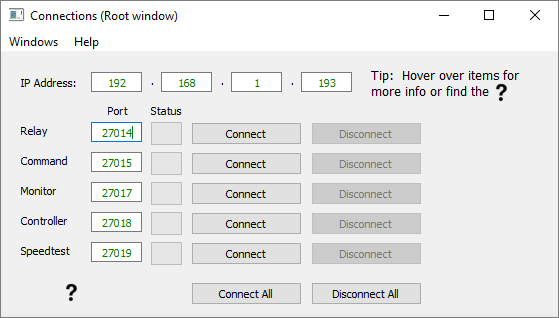
The root window allows you to individually connect to the different sockets on the SWTS ethernet board. Closing the root window closes the application. If you close one of the other windows, they can be brought back up from the "Windows" menu.
Data Received
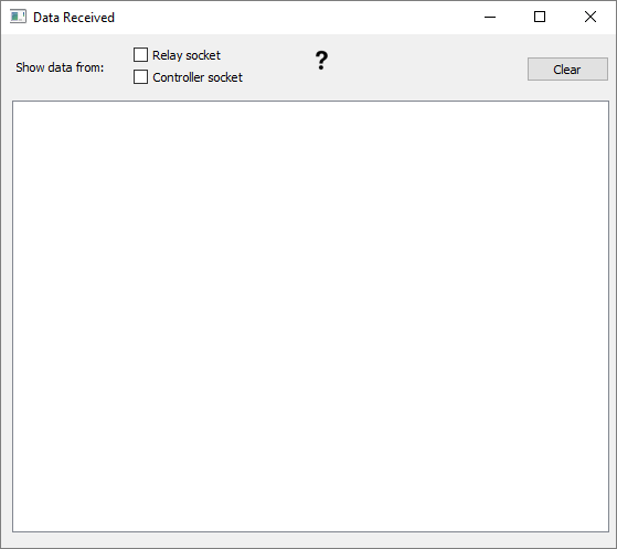
This window can be use to display any data received back by the GUI app. You may view data from either the relay socket or the controller socket. Make sure you are connected to the appropriate socket in the root window before attempting to view any data.
Speed Test
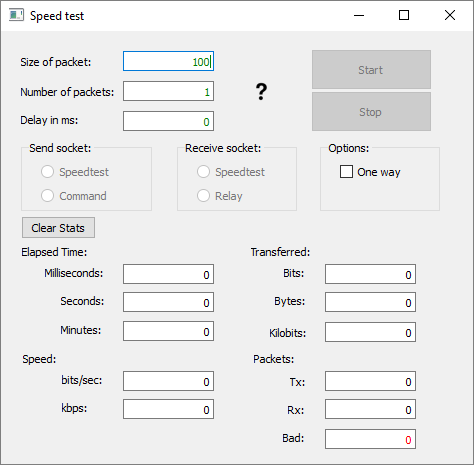
This window is used to conduct a speed test of the SWTS ethernet board. To conduct a speed test, first select which socket you want to send packets out of. Then, select which socket you want to receive packets on, then click "Start". Click "Stop" to end the test.
Results of speed test
Send Socket Receive Socket Loop back Result in kbps SWTS to SWTS Result in kbps
Speedtest Speedtest 164 110 Speedtest Relay 88 67 Command Speedtest 66 48 Command Relay 69 47
Commands
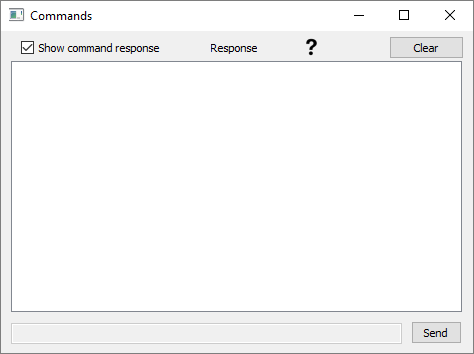
This is where you may enter SWTS commands that will be sent to the SWTS ethernet board. If the command is valid SWTS_OK response should be received.
SWTS Monitor
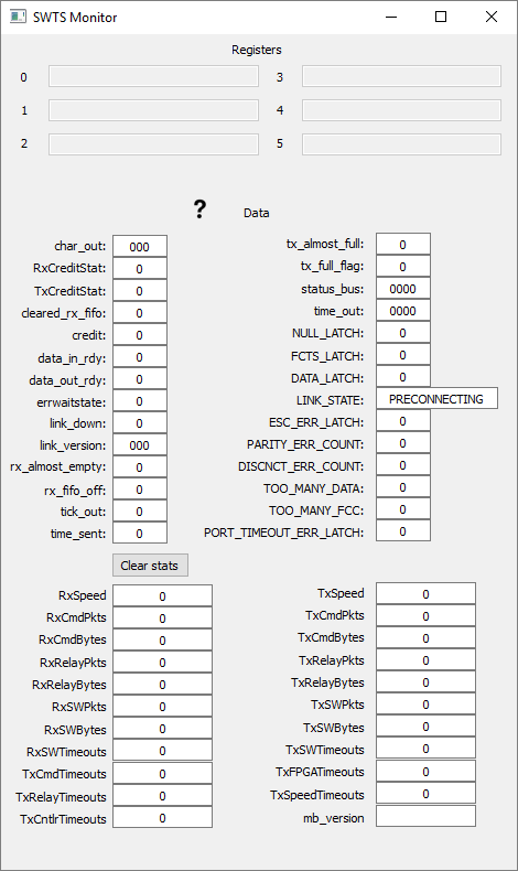
This window displays data about the SWTS ethernet board. All the data in this window is contained in a SWTS status packet that is sent once per second. The "Register" section shows the hex value of the six different registers. The "Data" section shows the data from the registers and displays each piece of data individually. The "Statistics" section shows the Rx and Tx values of the spacewire link along with some useful counts.
Controller
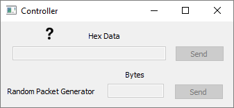
This window utilizes the controller socket. This can be used to send data to the SWTS ethernet, bypassing the command socket. Data is sent in binary form.
A loopback test connector is provided for easy setup and verification of operations.
In order to connect to the SWTS, your computer must be on the same subnet as the SWTS board. The IP of the SWTS board is 192.168.1.193, your computer must be on the 192.168.1.100 subnet. In Windows, open control panel, go to network and sharing center and select "change adapter settings" in the side bar. Right click on the local area network and select "internet protocol version 4" from the list. Change the ip to one on the 192.168.1.100 subnet and click "ok".
Commands and data packets are sent to the SEB via a command socket. Command and data are sent in ascii for simple operation. The commands are:
if (!strcmp(words.words[1], "PORTSPEED")) return SWTSOP_PORTSPEED;
PORTSPEED
This command shall configure the speed of the SpaceWire port. Command
Format: "SWTS PORTSPEED <portNum> <portSpeed>"
<portNum> is a required parameter. The format is ASCII decimal.
The value must be between „1‟ and „4‟.
<portSpeed> is a required parameter. The format is ASCII
decimal. The value represents the port Speed in Megahertz (MHz).
PORTUP This command shall cause the SWTSv2 to attempt to bring up
the port specified on the command line. Command Format: "SWTS PORTUP
<portNum>" <portNum> is a required parameter. The
format is ASCII decimal. The value must be between „1‟ and „4‟.
PORTDN
This command shall cause the SWTSv2 to bring down the port specified on
the command line. Command Format: "SWTS PORTDN <portNum>"
<portNum> is a required parameter. The format is ASCII decimal.
The value must be between „1‟ and „4‟.
RXRELAY2
This command behaves exactly the same as RXRELAY, except that it does
not strip the selected packets from the receive stream, it duplicates
them. Command Format: "SWTS RXRELAY2 <rt1>...<rtN>"
JWST-HDBK-003997 Revision Q 4-15 CHECK WITH JWST DATABASE AT:
https://ngin.jwst.nasa.gov/ TO VERIFY THAT THIS IS THE CORRECT VERSION
PRIOR TO USE. Use or disclosure of data contained on this page is
subject to the restriction(s) on the title page of this document.
rt1>..<rtN> value of Routing Byte(s) of packets to be stripped
from the received packet stream and relayed to the remote computer
system. The user may specify from 1 to 10 unique SpaceWire addresses for
relaying. The value of 0 will cause the SWTS to stop relaying all
packets. A value of „FF‟ will cause all received packets to be forwarded
to the relay socket. (Note: 'FF' will not work properly in applications
where the attached SpaceWire equipment can send data continuously at
more than a few Mbps) For high-speed applications use RXFILE to capture
data and analyze it after the fact
CLRCNTS
This command clears all status counts on the SWTSv2. Command Format:
return SWTSOP_ECLIPSECFG;
TXPKT
This command shall configure the SWTSv2 to transmit a single packet one
or more times. Command Format: "SWTS TXPKT <portNum> -p(s)
[-L] [<loopCnt>]" <portNum> is a required
parameter. The format is ASCII decimal. The value must be between „1‟
and „4‟, and indicates from which physical port the packet will be
transmitted. -p(s) is a required parameter. It denotes the beginning of
the packet definition. „-ps‟ shall cause a four octet sequence number to
be appended to the end of each packet. „-p‟ does not cause a sequence
number to be appended to the end of the packet. is a required parameter
set. It is essentially the packet to be transmitted represented as a
string of ASCII-hex bytes separated by spaces. The bytes shall be
transmitted onto the SpaceWire in the same order as they are entered on
the command line. [-L] is an optional parameter. It is used to include
a loop count with the packet definition. [<loopCnt.] is an optional
parameter that defines how may times to transmit the defined packet.
Command Result: The transmitter shall transmit the defined packet out
the specified port. If the --L option is used, the same packet shall be
transmitted <loopCnt> times. If the --L option is not present,
the packet shall be transmitted once.
Board Layout

Four discrete LEDs are installed on the board and can be used to display the status of the internal logic. These LEDs are attached as shown below and are lit by forcing the associated FPGA I/O pin to a logic '1' and are off when the pin is either low (0) or not driven.
LED Name Corresponding Board Label FPGA pin #
FPGA_GPIO_LED1 D1 J13 FPGA_GPIO_LED2 D2 K14 FPGA_GPIO_LED3 D4 U17 FPGA_GPIO_LED4 D5 U18
1 LED after power on 1 LED after program is loaded and running 1 LED for Command Socket connect 1 LED for Relay socket connect.
Development is using Xilinx ISE version 13.?
Signals brought to externals pins: DataRx => J5 PMOD1 P1 StrobeRx => J5 PMOD1 P2 DataTx => J5 PMOD1 P3 StrobeTx => J5 PMOD1 P4
Connector Pin Signal Name Board Pin
1 Din+ T6 2 Sin+ R7 3 Inner Shield GND 4 Sout- V5 5 Dout- P6 6 Din- V6 7 Sin- T7 8 Sout+ U5 9 Dout+ N5
Libraries/documents/LX16laoder
Eclipse Status Packet
SWTS Status Registers
::Once / second read and display registers 1,2 & 5.\
:
:   RxCreditStat =\> swts_reg2(29 to 31), 0 - 7\
:   TxCreditStat =\> swts_reg2(26 to 28), 0 - 7\
:   char_out =\> swts_reg1(0 to 9), display as hex\
:   cleared_rx_fifo =\> swts_reg2(25), 0 - 1\
:   credit =\> swts_reg2(24), 0 - 1\
:   data_in_rdy =\> swts_reg2(23), 0 - 1\
:   data_out_rdy =\> swts_reg2(22), 0 - 1\
:   errwaitstate =\> swts_reg2(19), 0 - 1\
:   link_down =\> swts_reg2(18), 0 - 1\
:   link_version =\> swts_reg2(10 to 17), 0 - ?\
:   rx_almost_empty =\>swts_reg2(9), 0 - 1\
:   rx_fifo_ff =\> swts_reg2(8), 0 - 1\
:   status_bus =\> swts_reg5(0 to 15), display in hex \-- breakout
    below\
:   tick_out =\> swts_reg2(6), 0 - 1\
:   time_out =\> swts_reg5(16 to 23), display in hex\
:   time_sent =\> swts_reg2(5), 0 - 1\
:   tx_almost_full =\> swts_reg2(4), 0 - 1\
:   tx_full_flag =\> swts_reg2(3) 0 - 1\
Register 5 STATUS_R(15) <= NULL_LATCH;"
STATUS_R(14) <= FCTS_LATCH;
STATUS_R(13) <= DATA_LATCH;
STATUS_R(10-12) <= LINK_STATE;
::::1 - ERROR RESET
:
:   2 - ERROR WAIT
:   3 - READY
:   4 - STARTED
:   5 - PRE CONNECTING
:   6 - CONNECTING
:   7 - RUN\
STATUS_R(9) <= ESC_ERR_LATCH;
STATUS_R(6-8) <= PARITY_ERR_COUNT(2); 0 - 7
STATUS_R(3-5) <= DISCNCT_ERR_COUNT(2); 0 - 7
STATUS_R(2) <= TOO_MANY_DATA;
STATUS_R(1) <= TOO_MANY_FCC;
STATUS_R(0) <= PORT_TIMEOUT_ERR_LATCH;\
The IP address of the board is 192.168.1.193.
SWTS Data Relay Socket
Connect to port 27014 for the SWTS Data Relay Socket. It works as defined in the SWTS User's Manual, section 4.3.3.
SWTS Command Socket
Connect to port 27015 for the SWTS Command Socket. It works as defined in the SWTS User's Manual, section 4.3.2. Not all SWTS commands are implemented, however. These are the implemented commands:
SWTS PORTUP SWTS PORTDN SWTS PORTSPEED SWTS RXRELAY3 SWTS TXPKT SWTS CLRCNTS
SpaceWire Controller Socket
Connect to port 27018 for the SpaceWire Controller Socket. This can be used for simple transmission of SpaceWire packets over Ethernet.
There are two kinds of packets that can be sent to the SpaceWire Controller Socket.
The first is a data packet. It contains an 8-octet header, followed by the raw bytes of a single SpaceWire packet. The first 4 octets of the header identify the packet type; they should all be 0. If an EEP packet need to be sent, those four octets should be 0x00 00 00 04 instead. The last 4 octets of the header should be the length of the SpaceWire packet, as an unsigned 32-bit integer. The SpaceWire packet should directly follow.
Updates must be requested by sending an Update Request. This should be four octets: 0x00 00 00 03.
When an Update Request is received by the board, it will respond with an Update Packet. An Update Packet has a 4-octet header, followed by a number of SpaceWire packets. The header contains the number of SpaceWire packets as an unsigned 32-bit integer. Each of the following SpaceWire packets are formatted with a 5-octet header followed by the raw SpaceWire packet data. The header starts with a 4-octet length field, which represents the number of bytes in the SpaceWire data as an unsigned 32-bit integer. The next octet is 0x00 if the packet was marked with EOP, and 0x01 if the packet was marked with EEP. It is then followed by the SpaceWire packet data. The SpaceWire packet data is immediately followed with the start of the next SpaceWire packet.
SEB Design Information
Implementation uses AVNET Xilinx Spartan-6 LX16 Evaluation Kit
Spacewire implementation based on GSFC Spacewire Link. Same IP core used in SWTS. Single Link with transmit data speed up to 200 mbps.
FPGA code developed in Xilink EDK versinon 13.2. Core is under project dslink. Microblaze interface is under project hw_design.
Microblaze processor implemented at 1.5 mbps. The board has 32 Mb x 16 (512 Mb) Micron LPDDR Mobile SDRAM component 128 Mb Numonyx Multi-I/O SPI Flash
XPS Etherlite core implemented for ethernet communications.
Microblaze flash bootloader implemented in FPGA. The bootloader is configured in wush.net SVN as SWTS_LX16_BSP and is version 67.
The Microblaze application code is stored in onboard flash memory and boots automatically when the board is powered on. The code provided reception of packet data via TCP/ethernet and forwarding on Spacewire, and Reception of packets on Spacewire nad forwarding on TCP/Ethernet. The current Microblaze code is configured under SVN as SWTS_LX16 and is version 103.
Telemetry Database Files
The telemetry database defines how to decode, transform, and interpret the various telemetry values contained in an instrument's packets.
Telemetry Database Fields
| Field | Required | Description |
|---|---|---|
| SUB_SYSTEM | Yes | The sub system that the telemetry value comes from |
| NAME | Yes | The name of the telemetry value |
| DESCRIPTION | Yes | A description of the telemetry value. Useful if the name is non-descriptive. |
| ADC # | Yes | Deprecated but still required right now, use 0 as the value |
| DATA_ID | Yes | The telemetry value's unique identifier |
| PACKET_TYPE | Yes | The type/APID of the packet that contains the telemetry value |
| PACKET_SUBTYPE | Yes | Deprecated but still required right now, use 0 as the value |
| DECODE_TYPE | Yes | The decode type, which dictates how the value is decoded, and also how decode ID 1-4 are used |
| DECODE_ID1 | Yes | The purpose of these depends on the decode type |
| RAW_FMT | Yes | How to format/display an unconverted telemetry value, i.e. the raw bits/bytes in the packet. Follows the C style printf formatting |
| ENG_FMT | Yes | How to format/display a telemetry value converted to its engineering representation. Follows the C style printf formatting |
| ENG_EQ_TYPE | Yes | The type of engineering transformation to apply to the raw value, and also dictates how the ENG_K1-ENG_K2 are used |
| ENG_K1 | Yes | Their usage depends on the ENG_EQ_TYPE, but is usually the coefficients of a 1st order polynomial. K1 = constant, K2 = coefficient of first order |
| SCI_UNITS | Yes | The units of the science transformation |
| SCI_FMT | Yes | How to format/display a telemetry value converted to its science representation |
| SCI_EQ_TYPE | Yes | The type of science transformation to apply to the raw value, and also dictates how the SCI_K1-SCI_K8 are used |
| SCI_FROM_ENG | Yes | If Y, then engineering transformation is applied to the raw value before science transformation. Otherwise, if N, then science transformation is applied directly to the raw value. |
| SCI_K1 | Yes | Values used in the science transformation. How they are used is determined by the SCI_EQ_TYPE. |
| DISCRETE_LABELS | No | Allows user to define a mapping of raw values to textual labels |
| MUX_CH | Yes | Deprecated but still required right now, use 0 as the value |
| LIMIT_TYPE_1 | Yes | The type of the first limit check |
| YELLOW_LIMIT_1 | Yes | The first limit check's yellow limit |
| RED_LIMIT_1 | Yes | The first limit check's red limit |
| LIMIT_TYPE_2 | Yes | The type of the second limit check |
| YELLOW_LIMIT_2 | Yes | The second limit check's yellow limit |
| RED_LIMIT_2 | Yes | The second limit check's red limit |
| EXTRA_1 | Yes | An extra field that is used for various purposes. |
Telemetry Metadata File
The telemetry metadata file is a new convention that was conceived during the MOMA project. Its main purpose is to store metadata about a telemetry file. However, its purpose may be extended in the future to include post processed data and perhaps other information. The original goal was to provide the ability to distinguish between the various instrument models. In other missions the file extension was used to determine the model, but after the patch file mechanism was adopted we lost this capability.
All versions will have their GSE metadata stored in the gse key. This allows us to easily add/remove/modify top level keys without breaking backwards compatibility and to also differentiate between items that are not necessarily GSE metadata.
Versions
Version 2
Fields
All fields from version 1 are carried over.
New
- default_mcal - The default mass calibration file that should be used to calibrate the science data. The mcal file should exist in the TID. In the rare case that it does not exist, MOMA Data View will attempt to use a different mcal file in the TID. If none exists, then it will attempt to copy one from the default mcal location. All other applications should quit with a message indicating the mcal file was missing in order to avoid misleading the user.
Example
{
  "gse":{
     "default_mcal": "2015-01-01-00.00.00-identity.mcal",
     "mission":"moma",
     "model":"etu",
     "patch_files":[
        "m1",
        "m2",
        "m3"
     ],
     "tid":534,
     "tid_dir":"2015-09-29-13.46.05-00534-",
     "tmfile_name":"tm.mom.m1.m2.m3",
     "version":1
  }
}
Version 1
Fields
- mission - Defines the mission for this data
-
model - Defines the model of the instrument that this telemetry
data was generated with. The model key is used to differentiate
between things that may differ between the various models, such as
the default mcal location or the SEB DAC table. The model's
corresponding entry in the 699config.ini file can be found by
combining the mission and model like
<MISSION>_<MODEL>. For example, for the MOMA mission and ETU model, its group in the 699config.ini file would be MOMA_ETU. - patch_files - This list defines the patch files that should be applied after the default database is loaded. They should be applied in the same order they are listed. The current convention is the corresponding patch file for a patch can be found in the TMDef directory and is in all caps with the ".txt" suffix. For example, for the m1 patch file, the text file can be found at momagse/TMDef/M1.txt
- tid - The test ID for this data
- tid_dir - The original TID directory that was generated
- tmfile_name - The telemetry file's name. This key can be used to determine the name of the telemetry file. If the telemetry file's name changes, this key should be updated.
- version - The version of the format
Example
{
  "gse":{
     "mission":"moma",
     "model":"etu",
     "patch_files":[
        "m1",
        "m2",
        "m3"
     ],
     "tid":534,
     "tid_dir":"2015-09-29-13.46.05-00534-",
     "tmfile_name":"tm.mom.m1.m2.m3",
     "version":1
  }
}
Time Synchronization Notes
The following was posted by Tom Nolan to Slack in November 2015.
The ExoMars rover doesn't use the SCLK terminology. In some other missions there is an SCLK, which is a counter onboard the spacecraft that counts up at some frequency. For those missions, you usually use a toolkit to convert SCLK to some usable time format.
The rover uses Rover Elapsed Time (RET), which is a 6-byte quantity: 4 bytes of seconds, and 2 bytes of subsecond ticks (65536 ticks = 1 second). They have not specified what time corresponds to 0 RET, but at some point they presumably will.
The FSW uses 3 different tick counts in various places: 100-microsecond ticks, 10-millisecond ticks, and 1-second ticks. The 100-us ticks start from power-on, because they're kept in a register in the FPGA. The other two start from FSW boot time, because they're kept in the flight software.
The telemetry packets contain 100-us ticks (what you're calling "FSW ticks"). The correspondence between ticks and RET is recorded in the digital status packet: whenever I get the time command from the rover, I record the RET contained in the command and the 100-us ticks when I got the command (a "time at the tone" concept). From this information, you can reconstruct the RET for each packet, but then you still need to do the RET-to-time conversion.
We're currently using a convention embedded in the EGSE for the RET-to-time correspondence (I think it's seconds since 1/1/2000, but I don't know for sure). But we need to anticipate that there will be other RET-to-time conventions when we integrate with the rover. I suspect that there is no requirement at the rover level to make RET unique. So during rover I&T, they will probably start RET=0 at power-on, and we'll potentially get data sets with overlapping times every time the rover is power-cycled.
There is also the possibility that RET will start over again at 0 on Mars, which would add to our headaches.
Tm2igor Quickstart
For Mac OS X:
- Install Python 3
- Install compiler
- Install Xcode from Mac App Store
- From Xcode, select Xcode/Preferences...
- Select Downloads then Components
- Install Command Line Tools
- Install python tools as described in PDL_Setup
- Close terminal window, and start a new one
- Download TMDef.zip
- Move TMDef.zip to the gse directory listed when you run:
- tmenv SAM gse
- cd to the gse directory
- unzip TMDef.zip
- cd into a TID directory (e.g. godata or tid #####)
- tm2igor.pl -d
- Enjoy your new IGORdata.zip file !!! ^_^
TunnelManager
General Information
TunnelManager is a graphical program for managing SSH tunnels to our various cloud-based hosts. It is a useful tool for those who want to use SVN but are still uncomfortable with the command-line. You will need access to the GSFC VPN and an account on the VME computers before you can use this program.
Releases
Version 0.2
Disk Image: tunnelmanager-0.2.dmg
Release Date: 2013-04-30
- First officially versioned beta release.
Updating mine699
This page details the steps to update the mine699 virtual machine.
If database changes break backwards compatibility, always make sure to update code before committing any database changes since mine699 auto updates the momagse repository when it processes new data!! If you don't, the mining process WILL break.
-
Build new extract_hk_data using the CentOS VM. Make sure to update the version number so that we can easily differentiate it from previous versions
-
Build new c699util library for both osx and centos (using the CentOS VM). Commit to their respective 699util repo locations
-
Build and release any applications that are affected by the code changes (MDV, 699util Python package, etc.).
-
Stop the mining process
-
Update the 699util repo on mine699 located at /mine699/scripts/labcode/699util-moma. Note: we use a developer's 699util setup on mine699, not the packaged distribution, so updating the SVN repo is all that is required to update the mining code.
-
Copy the new extract_hk_data to mine699:/mine699/scripts (hmmm maybe we should start committing this to the momagse dir so we can just update it from there instead of having to manually copy it)
-
Commit any database changes (some of which may depend on the new code changes)
-
re-enable mining process
-
Notify users of updated apps. Let them know if updating their apps is required for the database changes!!